A new curated data package focused on Housing and Community Development Finance is now available for license from PolicyMap. Drawing on more than 80 U.S.-based data sources, the collection covers...
The post New Data Package: License PolicyMap’s Housing and Community Development Finance Data appeared first on PolicyMap.
NYS GIS Association Membership Drive 2026–2027 (The Future is Spatial – be part of the NYS GIS Association!) Whether you’re a student, GIS professional, educator, developer, analyst, researcher, or decision-maker, the NYS GIS Association is the premier community for geospatial professionals across New York State. It offers opportunities to build connections, expand your knowledge, and […]
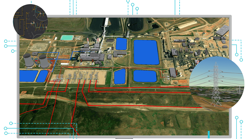
Most forestry companies, government agencies and insurers can produce a burn severity map. The harder part is delivering it quickly enough to support decisions, at scale when several fires are active, and accurately enough to trust when operational or financial consequences are immediate.
Dear NYS GIS Community, We are pleased to announce the launch of the website for the 2026 New York State GeoSpatial Summit, October 6–7, 2026 in Skaneateles, NY. 2026 NYS GeoSpatial Summit Website Here you will find further details regarding the: Preliminary presenter/panelist lineup Logistics info for venue, lodging, etc. Registration information (sign up by […]
A new job has been added to the NYS GIS Association website. Visit the GIS Job Postings page to view GIS jobs. When you think GIS jobs in NYS, think NYS GIS Association!
Geomatics is a diverse and interdisciplinary field that is constantly evolving and demanding new skills of GIS professionals as new technologies emerge. However, this is not reflected in the Government of Canada’s National Occupation Classification [...]
The post Why Canada’s GIS Profession Needs Modernized NOC and CIP Codes appeared first on GoGeomatics.
Introduction AI is everywhere. ChatGPT, Google Gemini, and Claude—names that barely existed in the public vocabulary a few years ago—now dominate headlines, boardrooms, and stock markets. But there’s another term quietly building the same kind [...]
The post How AI and GIS Are Transforming Critical Mineral Exploration in Canada appeared first on GoGeomatics.
GoGeomatics
• By Volunteer Editors and Group Writers
•
Every week, GoGeomatics contributors and editors review geospatial stories from around the world and select developments we think deserve the attention of the Canadian geospatial community. This week, several of the stories that caught our [...]
The post International Geospatial Digest – July 22, 2026 appeared first on GoGeomatics.
Prologis today announced the promotion of Travis Harvey to Global Head of Development, where he will lead Prologis’ global development and construction platform across the Americas, Asia and Europe. Harvey brings more than 20 years of industry experience to the role, including 11 years at Prologis. He has assumed the responsibilities of Greg Bauer, who recently […]
ST. LOUIS (July 21, 2026) — Saint Louis University has launched a new center focused on advancing geospatial research, fostering collaboration and developing solutions that benefit communities here at home and around the world. Housed in SLU’s School of Science and Engineering, the Geospatial Center will bring together faculty and students from across the University […]
AESPP strengthens collaboration between the European Union and Africa in space technologies, services and applications, helping expand the use of space-based solutions to address development priorities across the continent.
German-engineered handheld system combines centimetre-precise positioning, automated laser measurement, and integrated on-device reporting with zero app or cloud dependencies.
LLMs are good with text and bad with coordinates, so they guess when asked where things are. Overture is testing whether map geometry itself can become the connective layer across data themes, giving AI a verifiable spatial graph to reason over. ORATOR, a prototype built by Overture member Wherobots, (led by Daniel Smith) generated 700,000 nodes and 1.2 million edges over the San Francisco Bay Area to see if the idea holds.
Geometry is the foreign key. If a place sits inside a building, the data already knows they are related. Nobody had to write that link by hand.
This effort is in the prototyping phase, and we want input from the Overture community before any of it hardens into a standard. The goal is a cross-theme knowledge graph that solves real problems for developers and AI engineers, not a clever demo.
A strategic pillar for AI readiness
Large language models process language well. Ask one to do raw coordinate math or reason about what is near what, and it starts to struggle....
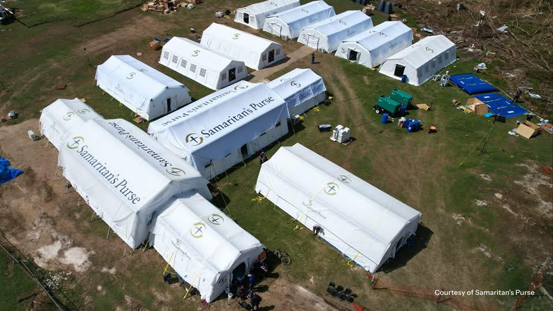
Hey guys, here’s this week’s edition of the Spatial Edge — a newsletter that’s as anticipated as The Odyssey. The aim, as usual, is to make you a better geospatial data scientist in less than five minutes a week.In today’s newsletter:Fine-Grained Damage Assessment: Drone AI improves post-disaster mapping. Remote Sensing Agents: RS-Claw streamlines AI tool selection. Cross-Border Generalisation: Foundation models struggle across countries. Night-Time Dataset: Sentinel-2 releases high-res nighttime imagery.Subscribe nowResearch you should know about1. Fine-grained damage assessment from drone imageryRapid and accurate damage assessment is pretty important after natural disasters, but manual field surveys are often too slow or can be too dangerous to conduct. So automated semantic segmentation models offer a faster alternative, yet they frequently struggle to provide the fine-grained detail required for effective emergency response. When researchers feed high-resolution drone imagery...
GeoFeeds Daily Briefing — Wednesday, July 22, 2026 Covering posts from 0800 ET July 21 to 0800 ET July 22. Sources: 162 geospatial feeds. Three Topics That Stood Out A moderate window dominated by the ripples from Esri's 2026 User Conference and by the independent Tier 1 voices. Three threads held together: what happens once foundation models are actually inside the platform, 3D reality capture settling into real workflows, and a sovereignty conversation that gained a hard-security edge. 1. Foundation models are in the platform now — the conversation shifts to operationalizing and governing them The GeoAI and the Law newsletter used Esri's 2026 User Conference announcement — that geospatial foundation models (NASA/IBM's Prithvi, the open Clay models, ESA's TerraMind) are becoming part of ArcGIS — to argue the legal questions have moved from theoretical to mainstream now that these capabilities sit inside tools thousands of analysts use daily. In the same window, Will Cadell...
Sovereignty: National Autonomy, Strategic Resilience, and Governance Models
How should nations redefine geospatial and space sovereignty in an era of increasing dependence on global platforms, foreign satellite constellations, and international data infrastructures?
Nations must shift their definition of sovereignty from “exclusive ownership of hardware” to “assured access to data and analytical autonomy.” True geospatial sovereignty means having the capacity to generate reliable ground-truth insights independently, continuously, and verifiably, regardless of geopolitical disruptions or weather conditions. This distinction is especially vital for middle-power nations.
At the same time, attempting to achieve this capability entirely within one’s own borders is not realistic for most countries. Except for a handful of great powers with overwhelming economic, technological, and military strength, it is no longer financially or technically feasible to achieve full...
Celia’s the person who got an entire generation of EAGLE students to care about ice they’ll probably never set foot on. She’s a postdoctoral researcher in the “Polar and Mountain Regions” team at DLR, and she teaches the EAGLE course “Earth Observation of Cold Regions”. This intensive block course takes students on a journey through Antarctica, the Arctic, and mountain regions around the world, with a particular focus on the Alps and many hands-on programming exercises.
After studying in Erlangen and Bonn, she did her PhD at the University of Würzburg, where she built a CNN-based algorithm to automatically detect glacier and ice shelf front positions from SAR satellite imagery, applied along the entire Antarctic coastline. That’s a genuinely tricky problem, ice fronts move, fracture and calve in ways that are hard to track manually at continental...
One of the biggest challenges when moving home is deciding which compromise you are prepared to make. You might want to live close to work, a good school, a supermarket, a park, a gym and your favourite coffee shop - but finding somewhere that sits within easy reach of everything is rarely possible.Close is an interactive travel-time map of the United States designed to solve exactly that
We had a really special visit at the University of Würzburg on July 16: Germany’s Federal Minister for Research, Technology and Space, Dorothee Bär, came to the Mission Control Center on Campus Hubland Nord by the Informatics Faculty, and we were glad to be part of the day.
The visit was organized around a talk Dorothee Bär gave to the general assembly of the IHK Würzburg-Schweinfurt on what research, technology, and space can do for the Mainfranken region. Fittingly, the whole thing happened right in the Mission Control Center run by Hakan Kayal, professor for space technology at the Institute of Computer Science. Dorothee Bär even got to send live commands to SONATE-2, the nanosatellite Kayal’s team put into orbit via a SpaceX launch back in 2024, which by the way was the first time Germany trained an AI on board a satellite in space.
Prof. Marco Schmidt – our collaboration partner e.g. in the Super-Test-Site Würzburg project – presented his group’s work on embedded systems and...
How can Earth observation support sustainable water management in times of climate change? This question was at the center of a recent visit by participants of the EAGLE block course “Linking Science and Practice in Earth Observation for Climate Adaptation” to the Department of Water Management at the Government of Lower Franconia. The visit offered a valuable opportunity to connect scientific approaches with real-world challenges in public administration. As part of the course, led by EORC staff Dr. Julian Fäth and Dr. Sarah Schönbrodt-Stitt, students presented posters showcasing different applications of remote sensing for climate adaptation. The first focused on land use classification as a basis for identifying and planning adaptation measures. The second explored the use of satellite data to analyze the phenology of deciduous forests in the Rhön region. The third demonstrated how remote sensing can be used to detect dried or intermittently flowing streams, an important aspect...
On July 24, 2026, Wajiha Yasmeen will present her inno lab results on ” Comparing intra-urban thermal patterns using high-resolution HotSat-1 and Landsat 8 data from 14 U.S. cities ” at 12:00 at the EORC meeting room/1st floor in John-Skilton-Str. 4a
From the abstract: Higher resolution thermal imagery is widely expected to improve the study of surface urban heat island effect, but this has rarely been tested directly against established sensors like Landsat. Therefore, we compared the relative thermal behavior of building and street types across 14 U.S. cities using sensor-specific normalized thermal indicators. Radiance from high resolution thermal satellite HotSat-1 and LST values from Landsat-8 were extracted for individual urban features using OpenStreetMap building and road polygons, and Getis-Ord Gi* hot and cold spot analysis was computed over both rasters to identify statistically significant thermal clusters. Because the two sensors record physically different quantities,...
Simon is the lecturer who teaches you what to actually do when a volcano starts erupting and someone needs answers in hours, not weeks. He is with the Natural Hazards team at DLR and runs the EAGLE MSc course “Risk and Disaster Earth Observation,” which is basically a crash course in turning satellite data into something useful while a disaster is still unfolding.
His day job is developing automated algorithms for extracting crisis information from optical, thermal and SAR imagery, and he is not just doing this from a research distance either. He is an Emergency On-Call Officer and Project and Data Manager for the International Charter “Space and Major Disasters,” and he works through DLR’s Center for Satellite based Crisis Information, ZKI, which feeds directly into national and international disaster response efforts. So when he is teaching students how rapid...
Laut Wikipedia [1] hat Downtown folgende Bedeutung: „Das Wort Downtown wird hauptsächlich in Nordamerika im Englischen verwendet, um die Innenstadt oder den zentralen Wirtschaftsbereich einer Stadt zu bezeichnen“. Soweit klar, wusste man, aber wisst Ihr auch, wo die Downtown in Eurer Stadt liegt? Auf X (ehem. Twitter) [2] habe ich jetzt eine Webanwendung gefunden, ich welcher der Nutzer sein Gefühl oder Wissen über die Downtown eintragen kann. Über alle Eintragungen wird dann live der Durchschnitt berechnet und als Hexagon-Karte angezeigt.
Screenshot 1: Meine Erfassung und das Ergebnis, die Downton in Halle (Saale)
Ich habe es natürlich für Halle (Saale) probiert, hier die Ergebnisse. Übrigens Hallenser, in Halle gibt es noch recht wenige Einträge, momentan nur sechs. Ihr solltet Euer Wissen oder Gefühl über Halle-Downtown einbringen. Also los, „Where is Downtown?“ [3].
Screenshot 2: Meine Erfassung und das Ergebnis, die Downton in Halle (Saale) über das gesamte...
Even though the conversations on climate change have muted due to the geopolitical situation, trade disruptions, greater defence and intelligence spending, and shift in key policies, the negative effects of climate change are being faced all over the world. This however, does not signal that we have stopped working towards a positive climate action.
To highlight and discuss an important aspect of urban heat mapping, we have with us Mr. Urmil Bakhai who is a business leader with over 22 years of experience turning early-stage ideas into market-leading organizations.
The post Mapping Urban Heat Islands in Ahemedabad appeared first on Geospatial World.
I keep watching the same thing happen. A company decides Earth observation is finally within reach, hires a data scientist or two, points them at some AI tools, and waits for the insight to arrive. For a few weeks, it seems to be working. Then reality lands. Lat/long is not as simple as two numbers. Ground truth is expensive and scarce. Cloud cover eats half the archive. The domain logic that a remote sensing specialist carries in their head turns out to be the whole game. The demo that impressed everyone does not survive contact with an operational question.
This is not a failure of talent or of ambition. It is a failure of translation. And it is about to define who wins in geospatial AI.
The models are not the problem
Every quarter brings a better foundation model for imagery, a sharper segmentation approach, a new way to reason over a scene. The capability is genuinely good. And yet most organizations sitting on decades of EO data still cannot ask an AI system a...
—Open Library on Green EconomyCan Himalayan Crops Help Secure the Future of Food?As we navigate the intensifying impacts of the 2026 El Niño, the vulnerability of our global food systems require careful evaluation. With this year’s erratic weather patterns driving severe, prolonged droughts in some regions and unseasonal, devastating floods in others, the climate crisis is proving that it is not a distant threat; it is happening rig…Read more4 days ago · 2 likes · Jeevan Labh ^^^^ shared technical post—Open Library on Green EconomyWhere Sustainability Meets ActionBy Akaash Dudwani ^^ shared Substack, “Open Library on Green Economy”—https://adaptationwithoutborders.org/knowledge-base/adaptation-without-borders/shifting-cooperation-in-the-hindu-kush-himalaya/ <-- shared technical article, “Shifting cooperation in the [HKH]”—https://www.icimod.org/who-we-are/the-hindu-kush-himalaya/ <-- background on the HKH, International Centre for Integrated Mountain Development...
Updated with graphics at bottom
Apologies in advance, this is unedited stream of consciousness
OK, we have talked about 3DGS for a while now on the podcast, from news items last year to full discussions in June (I think). For the most part, I have stuck with traditional structure-from-motion/close-range photogrammetry in my day to day processing and use. I had students do collection using Scaniverse, RealityCapture (now RealityScan), or similar app to get a sense of what could be done, but I didn’t really use it.
But, things changed as processes became more streamlined and conversations continue to grow. We at VerySpatial have always leaned a little toward the geovisualization side, so it was probably inevitable we would take our different approaches to gaussian splats. I even waited impatiently through the spring until education site licenses got access to esri’s reality capture tools to see how they compared to some of the open source and trial software that I had moved...
--https://doi.org/10.1029/2026EF008578 <-- shared paper--https://www.thearcticinstitute.org/climate-change-geopolitics-monitoring-thawing-permafrost/ | https://www.thearcticinstitute.org/dwindling-arctic-sea-ice-impacts-permafrost-health/ <-- shared technical articles--https://www.theguardian.com/cities/2016/oct/14/thawing-permafrost-destroying-arctic-cities-norilsk-russia <-- shared media article--https://news.grida.no/new-map-shows-extent-of-permafrost-in-northern-hemisphere <-- shared technical article--H/T “Why the increase?Our understanding of climate risk is only as good as our understanding of our exposure to hazards. The better we can account for what is at risk, the better we can measure risk in a changing world.In this new study [link above], [they] investigate[d] how damage to the building stock across the Arctic, a key impact of permafrost degradation, is underestimated because of underdeveloped exposure information. With National Science Foundation (NSF) supercomputers...
Welcome to the 147th issue of Geospatial Jobs, a newsletter focusing on data science and geosciences (🌧climate-tech, 🌽ag-tech, 🌊risk modeling, ⚡️energy, 🛰remote sensing, ♻️sustainability, and more).The paywall on issue #143 is removed and it’s now freely accessible. Shout out to Apoorva Shastry and Manjaree Binjolkar who voluntarily helped with formatting this issue.Share🕵️💵 Recent Fundraisings / Updates:Nothing relevant this week.💡📚 Useful Resources:Nothing interesting this week.PhD positions:JHU: 2 positions on climate variability, human impacts & resilienceFlorida International U: 2 positions on AI & ML for urban water systems & sewer modellingU Houston: AI & remote sensing for land-atmosphere interactions & coastal resilience🇨🇭ETH Zurich:SAR remote sensing for Arctic permafrost monitoringGlobal trade, supply chains & climate shock propagation🇨🇭U Neuchâtel: Remote sensing & drone imagery for tropical forest structural monitoring🇪🇸 IDAEA-CSIC: Air quality monitoring &...
GeoAI and the Law Newsletter
• By Spatial Law & Policy
•
GeoAI and the Law is not legal advice. The reader should consult with a trained lawyer on legal matters associated with GeoAI.Deep DiveGeospatial Foundation Models Have Arrived — And the Legal Questions Came With ThemFor the last couple of years, I’ve been exploring the complex legal issues that will arise as geospatial foundation models are integrated into existing geospatial workflows. Last week, that that future took one step closer to becoming a reality. At its 2026 User Conference, Esri announced that foundation models are becoming part of ArcGIS. Geospatial models such as NASA and IBM’s Prithvi, the open Clay models, and ESA’s TerraMind have been maturing for a while. But as these capabilities become part of a platform used daily by thousands of geospatial professionals, accessible through the same tools analysts already use, the legal questions move into the mainstream.So, it’s worth stepping back and asking why a geospatial foundation model changes the legal calculus.What...
FME Blog - FME by Safe Software
• By Julie-Alisson Ducros
•
This work was done in collaboration with Safe Software partner Graphland.
At BIM World 2026 in Paris, Safe Software partner Graph Land presented a workflow connecting site surveys, BIM modeling, and on-site visualization, with FME Realize playing one specific role: bringing project data back to the field.
The problem: data that doesn’t talk to itself
On a renovation or construction-monitoring project, data piles up fast: point clouds from laser scans, existing DWG drawings, IFC models, GIS layers, and field surveys. Each tool does its job well, but the formats don’t communicate with each other. The result: models disconnected from the actual site, time-consuming manual back-and-forth between software, and data that teams stop trusting the more it passes from one tool to another.
This was the challenge Graph Land explored during its workshop at BIM World 2026, led by Julie-Alisson Ducros. Rather than looking for a single tool meant to cover...
The survey programme will support the planning and development of critical offshore energy infrastructure associated with the Greater Sunrise and Bayu Undan developments, two strategically important projects that underpin Timor-Leste’s future energy ambitions. Under the contract, Fugro will undertake an extensive offshore site characterisation programme, including geophysical, seismic and autonomous underwater vehicle (AUV) surveys across […]
28th Offshore China (Shenzhen) Convention 2026 (OC2026) was held in Shenzhen on June 16–17, themed Venture Deep Seas, Drive Industrial Upgrade: Accelerate High-Quality Offshore Energy & Equipment Development, with a parallel core agenda Foster Win-Win Collaboration & Build Resilient Industrial Ecosystem. The event gathered senior representatives from leading global oil operators including CNOOC, Petronas, Petrobras, […]
Members spanning technology, public sector, academia and non-profits standardize on open spatial data and unique IDs via GERS. Overture Maps Foundation, a collaborative effort to build a foundational base layer of map data to facilitate data exchange, announced it has reached 50 members, nearly doubling its 2024 count, as more industries turn to open spatial […]
Silicon Sensing has launched its latest gyro, delivering unmatched reliability in harsh environments. The CRG21 is Silicon Sensing’s latest compact micro electro-mechanical systems (MEMS) gyroscope. This closed-loop, single-axis rate sensor is a direct replacement for the company’s highly successful CRG20 gyro, already proven in several key inertial systems. Engineered to operate in harsh conditions, this […]
How Integrating Laser Trackers and Modular Arms Creates a “Unified Nervous System” for Complex Alignment and Calibration By Mark Shotwell, Senior Field Applications Engineer, FARO CREAFORM When an aerospace engineer oversees the assembly of a 30-meter fuselage, or a plant manager verifies the alignment of a massive carpet-tufting machine with thousands of precisely synchronized […]
The survey programme will support the planning and development of critical offshore energy infrastructure associated with the Greater Sunrise and Bayu Undan developments, two strategically important projects that underpin Timor-Leste's future energy ambitions.
GeoFeeds Daily Briefing — Tuesday, July 21, 2026 Covering posts from 0800 ET July 20 to 0800 ET July 21. Sources: 162 geospatial feeds. Three Topics That Stood Out A busier window than the mid-summer weekend that preceded it, with the independent voices and Tier 1 analysts back in force. Three threads held the day together — one on where the AI conversation is actually heading, one on sovereign tooling, and one looser thread about the ground literally moving under the data. 1. The AI-and-GIS conversation splits into building, believing, and grounding Three feeds approached AI from different altitudes on the same day. Will Cadell (Strategic Geospatial) started building a geospatial analyst assistant in the open, deliberately framing it against the usual "dopamine-fueled, token-burning" sprint and treating it as a disciplined engineering project. GoGeomatics published a GeoIgnite 2026 interview with Peter Rabley advancing a "Total World Model" and "Adequate AI" as Canada's strategic...
Los datos son el motor de la revolución tecnológica que supone la IA. En el ámbito de los Sistemas de Información Geográfica (SIG), la ética de los datos adquiere una importancia especial porque los datos espaciales pueden revelar información muy sensible sobre personas, comunidades y el medio ambiente. A modo de introducción De forma habitual ...
Leer más
Ética de los datos en los SIG: privacidad, sesgos y buenas prácticas en la era de la Inteligencia Artificial
Spatialists – geospatial news
• By Ralph Straumann
•
A consortium of 60 Swiss firms has secured funding to build AV-QGIS, a specialist #QGIS module for #cadastralSurveying built around the new #DMAV data model, with basic data updates due by 2028 and full rollout by mid-2028. It’s a welcome sign of competition and sovereign, #openSource alternatives in the #surveying software space.
Shinjuku Station has a well-earned reputation as one of the world's largest and most bewildering transport hubs. The Shinjuku Station Indoor interactive 3D map tackles that complexity by turning the station's official indoor mapping data into a clean, schematic three-dimensional blueprint. This map strips everything back to the essential geometry of corridors, platforms and rooms, making
Our profession’s future needs not only better tech, but stronger leadership, collaboration and research translation.
The post Connecting geospatial innovation to real-world impact appeared first on Spatial Source.
The local council area in Perth’s northern suburbs is now more accessible thanks to a new footpath mobility map.
The post Wanneroo makes life easier with new mobility map appeared first on Spatial Source.
The next Joint Urban Remote Sensing Event – JURSE 2027 (https://jurse.org/) will be held in Amsterdam, The Netherlands from the 30th of June to the 2nd of July 2027 (https://www.jurse2027.org/). The Joint Urban Remote Sensing Event – JURSE has always been one of the most important international conferences for our work at EORC and DLR – see e.g. here: https://remote-sensing.org/contributions-to-the-joint-urban-remote-sensing-event-jurse-2025-1/ or https://remote-sensing.org/contributions-to-the-joint-urban-remote-sensing-event-1/
It will again be an excellent opportunity to meet researchers, practitioners, and students working in urban remote sensing. JURSE introduces new methodologies and technological resources to investigate urban environments through orbital and airborne remote sensing.
Now, the Call for Papers has been published – https://www.jurse2027.org/call%20for%20papers/ . JURSE welcomes submissions on all topics related to urban remote sensing. Submissions can be made...
The new NSW Bionet Atlas map viewer provides easy access to multiple fauna and flora data collections.
The post Environment and Heritage’s BioNet Atlas map viewer appeared first on Spatial Source.
Screenshot: Selbstversuch – Der #geoObserver als Satellitenbildermosaik
Im April hatte ich hier in „Cool: Dein Name aus Satellitenbildern“ [1] darüber berichtet, wie man aus realen Satellitenbildern Schriftzüge erstellen kann. Nun habe ich in der Wochennotiz 834 [2] einen Beitrag mit einer Anwendung gefunden, die auch reale Satellitenbildern, diesmal von „Sentinel 2“ verwendet. Hier werden die Satellitenbilder genutzt, um hochgeladene Bilder in einer Browser-App als Mosaik einzufärben. Navigiert Ihr durch das Ergebnis, zeigt die App auf jedem Mosaik-Teilchen die reale Szene in der Welt inkl. den Koordinaten. In jedem Fall interessant und unterhaltsam. Ihr findet alle Details unter „Sentinel-2 Paint: Recreate Any Image from Real Satellite Imagery“ [3] und könnt die App unter Sentinel-2 Paint [4] starten. Ich habe es mal im Selbstversuch ausprobiert und es funktioniert perfekt
Animation: Jedes #geoObserver-Mosaikteilchen ist ein reales Satellitenbild
[1] …...
How do the municipalities in the Lower Franconian Main valley deal with flooding and heavy rainfall?
This question was the focus of a working meeting of the Remote Sensing and Social Geography working groups on July 15, 2026, for the “MainPro” research project (Ecosystem-based solutions for hazard scenarios). Prof. Dr. Jürgen Rauh, Prof. Dr. Hannes Taubenböck, and Tobias Riemann, M.Sc., came together to link the previous findings from the spatial geodata analysis with the qualitative investigations of the project and to evaluate the next steps.
The social geography work package, which also forms the core of Tobias Riemann’s dissertation, was the center of attention at the meeting and provides insightful glimpses into the reality of municipal planning. Based on detailed risk maps, particularly vulnerable municipalities were specifically selected in advance for in-depth interviews.
In addition to presenting the initial findings from these interviews, another focus of the meeting was...
The program to modernise New Zealand’s land titles and survey system has come in on time and under budget.
The post NZ’s Landonline modernisation project praised in report appeared first on Spatial Source.
--https://doi.org/10.1111/gwat.70092 <-- shared paper--H/T @ThomasWöhling | Professor at TU Dresden“Do you like braided rivers? We think they are soooo beautiful. And they are interesting to study as well. Particularly how these complex and transient systems interact with regional aquifers…”--“Coupled models of two braided rivers with real, pre- and postflood event morphologies are studied for river–groundwater exchange changes…”--“Braided river systems are an important source for groundwater recharge, but their complex morphology makes river–groundwater exchange fluxes difficult to estimate. Their river channel morphology changes frequently after floods, which has effects on recharge rates that have rarely been studied in the past. This work aims to isolate the effects of changes in braided river morphology on groundwater recharge for two sections of the Wairau River and Waikirikiri River in New Zealand. For each study site, two different river morphology variants of a fully coupled...
--https://memolaproject.eu/sierra-nevada/wateruse <-- shared link to the 𝗠𝗘𝗠𝗢𝗟𝗔 𝗣𝗿𝗼𝗷𝗲𝗰𝘁 page--https://regadiohistorico.es/ <-- shared technical page, “Collaborative map of historical irrigation systems in Granada and Almería” / “Mapa colaborativo de regadíos históricos de Granada y Almería”-- <-- shared video overview, “Participa al Mapa colaborativo de regadíos históricos de Granada y Almería”--H/T @Sofie de Volder | Co-founder TRAQUA • Flooding your feed with groundwater stories • Aquaholic💧• Hydro(geo)logy, dye tracing 🧪, karst“[The author has] already discussed ancient water management systems, such as the qanats in Persia and other Eastern countries. In Europe, there are the acequias of the Sierra Nevada in Andalusia, Spain.The hand-dug channels date back over 1,000 years to the Moorish era. Networks of canals, aqueducts and cisterns were engineered to capture and transport snowmelt, turning this natural resource into a sustainable water supply for agriculture. The...
--https://www.ordnancesurvey.co.uk/news/new-biodiversity-tool-in-scotland <-- shared technical article--https://biodiversity.scot/ <-- shared Farm Biodiversity Scotland (FarmBioScot) home page--https://www.nature.scot/ <-- shated NatureScot home page--H/T @Ordnance Survey“Most of us use maps to find places. Farmers in Scotland are now using them to help restore nature. 🌿A new tool from NatureScot powered by Ordnance Survey data, is being tested with farmers and crofters and helps them map habitats, record wildlife observations and track biodiversity improvements across their land.By turning trusted location data into practical insights, FarmBioScot makes it easier to understand the environmental value of the land they manage, support nature recovery and meet requirements for The Scottish Government support schemes.It’s a great example of how geospatial data can help people make better decisions - benefiting both rural businesses and the natural environment…”--“NatureScot, Scotland’s...
The PostGIS Team is pleased to release PostGIS 3.7.0beta1!
Best Served with PostgreSQL 19 Beta2
and GEOS 3.15.0beta2.
This version requires PostgreSQL 14 - 19beta2, GEOS 3.10 or higher, and Proj 6.1+.
To take advantage of all features, GEOS 3.15+ is needed.
To take advantage of all SFCGAL features SFCGAL 2.3.0+ is needed.
This release contains fixes and enhancements since 3.7.0alpha1 release.
3.7.0beta1
source download md5
NEWS
HTML Online en ja zh_Hans fr
PDF docs: en ja, zh_Hans, fr
Cheat Sheets:
postgis: en ja zh_Hans fr
postgis_raster: en ja zh_Hans fr
postgis_topology: en ja zh_Hans fr
postgis_sfcgal: en ja zh_Hans fr
This release is an alpha of a major release, it includes bug fixes since PostGIS 3.7.4 and new features.
GeoIgnite 2026, Canada’s national geospatial leadership conference, was held in Ottawa from May 11 to 13. It brought together leaders from government, industry, academia, Indigenous organizations and international partners to discuss the role of geospatial [...]
The post Peter Rabley on the Total World Model, Adequate AI, and Canada’s Window appeared first on GoGeomatics.
In most parts of the world, the ground beneath a construction site can be treated as a fixed and stable reference point. You dig, you install, you backfill, and the infrastructure stays where you put it. In permafrost regions which span vast stretches of Alaska, Canada, Russia, and the broader Arctic, that assumption does not hold.
What Is Permafrost and Why Does It Matter?
Permafrost is ground that remains frozen for at least two consecutive years. More than 80% of Alaska, 50% of Canada, and 65% of Russia sit on it, with roads, pipelines, buildings, and buried utility networks all depending on it staying frozen and stable. When permafrost thaws, the ground subsides, and buried infrastructure shifts position because the ground itself has moved. It is one of the only environments in the world where a utility record can become inaccurate without anyone touching the infrastructure.
How Has Construction Traditionally Handled It?
Arctic engineers have spent decades...
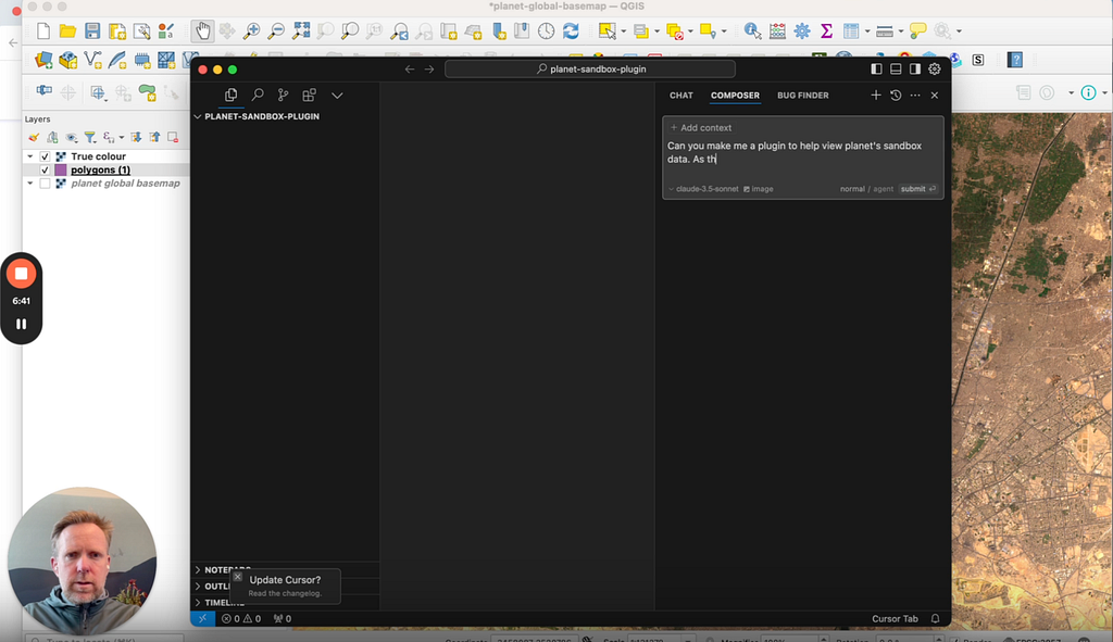
I’ve started building again. Not in the way I used to, but it’s not wildly different either. In fact, I can now build alongside my day job.Photo by Valentin Petkov on UnsplashI am building an assistant. At some point, it will be a fully fledged Geospatial Analyst. Today, it's just a tool I can use to ask questions and quickly source and view our changing planet. This is something I have been wanting to do for some time. I will do this somewhat openly, so you can play along too. As we do this, I’ll be evaluating a series of tools and practices. Hopefully, we’ll be left with a sense of what is working these days and what might still be flaky.Strategic Geospatial is a reader-supported publication. To receive new posts and support my work, consider becoming a free or paid subscriber.Something that I know is flaky is how people go about these projects. There is typically minimal planning, and feature bloat tends to follow a dopamine-fueled, token-burning few hours. So, it’s worth taking a...
Telecom operators are expected to invest an average of $87 million in autonomous networks by 2030, according to Capgemini*. While much of the industry focus is on AI and automation, these investments raise a more fundamental question: what will those systems actually rely on to operate effectively?
On July 21, 2026, Wajiha Yasmeen will present her internship results on ” Detection of Off-The-Road Tyre Dumpsites at Mining Operations Using Sentinel-2 Imagery and Deep Learning Segmentation ” at 12:00 at the seminar room 3 in John-Skilton-Str. 4a.
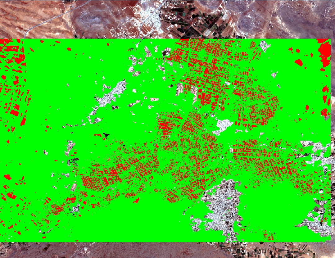
From the abstract: Discarded off-the-road (OTR) tyres at mining sites represent a persistent environmental hazard, yet their locations are poorly documented across large mining regions. This work develops a supervised semantic segmentation pipeline to detect OTR tyre dumpsites from Sentinel-2 multispectral imagery across mining operations in Chile. Per-mine Sentinel-2 composites were exported and candidate dump areas identified through spectral thresholding, then manually verified and digitised in QGIS. A DeepLabV3+ network with a pretrained encoder was trained on 10-band input using a combined Dice and weighted binary cross-entropy loss. Results indicate that site-level detection is achievable with the current approach, while accurate...
Trimble Financials, a simplified accounting and job costing solution, now available as standalone subscription or within software packs for MEP, civil and general contractors WESTMINSTER, Colo., July 20, 2026 — Trimble today announced the availability of Trimble Financials™ software in the United States. The new construction-specific financial management and job costing solution is designed to […]
Geospatial Frontiers - Project Geospatial
• By Adam Simmons
•
SERIES FEATURE
EDITORIAL SPECIAL // 2026 GEOSPATIAL REGIONAL HUBS
Geospatial Regional Hub Article Series
This installment is part of an ongoing investigative series analyzing the nation's premier mapping and spatial intelligence hubs. Each deep dive evaluates the strategic interplay between national security imperatives, civilian commercial applications, academic geocomputation, and the local socioeconomic infrastructures driving regional technology corridors.
Explore Series
...
GeoFeeds Daily Briefing — Monday, July 20, 2026 Covering posts from 0800 ET July 19 to 0800 ET July 20. Sources: 162 geospatial feeds. Three Topics That Stood Out A quieter mid-summer window, one notch above a dead weekend — the trade and analyst feeds are still coming back from the Esri UC hangover, but the independent voices showed up. Three loose threads held the day together. 1. AI segmentation reaches the plugin panel Two feeds, from opposite ends of the pipeline, put deep-learning segmentation to work on imagery. geoObserver spent the weekend hands-on-testing TerraLab's new "AI Segmentation" QGIS plugin, running building- and tree-detection on Saxony-Anhalt DOP 20 orthophotos and writing results straight to a GeoPackage. In parallel, an EAGLE internship writeup detailed a Sentinel-2 plus DeepLabV3+ pipeline to detect off-the-road tyre dumpsites across Chilean mining sites. Different worlds — a FOSS blogger clicking through a plugin, an academic training a segmentation network...
I am an inveterate infrastructure geek due to work I did earlier in my career in critical infrastructure protection. One of my projects was to build a system to model the behavior of commercial freight rail. Of course, I am also a programmer. Between railroads and writing software to model them, it was impossible to avoid dealing with time zones, so I inevitably also turned into a time zone geek. If you join me in that elite club, then 2026 is shaping up to be our year.
This October, the General Conference on Weights and Measures, the world’s authority on measurement, will decide how quickly civil time should stop chasing the uneven rotation of the Earth. The immediate problem is that the planet has recently been rotating fast enough to raise the possibility of the first negative leap second. Adding an occasional second is already disruptive. Removing one, something no production timekeeping system has ever had to do, is considerably worse.
You can be forgiven if you haven’t...
We got to sit in on something really special during our 10 year of EAGLE anniversary: a plenary discussion with four EAGLE alumni, moderated by Will, one of our 10th generation students. And honestly, it was one of those sessions where you look around the room and just feel the energy. Four very different career paths, one shared starting point.
On the panel we had Sofia, Yomna and Magdalena, all three currently pursuing their PhDs, and Karsten, who took a different route and founded his own company, supervision.earth. Four people, four directions, but all of them EAGLEs first.
Will steered the conversation with questions that got past the small talk pretty quickly. What actually inspired you during EAGLE? What’s the one memory that still sticks with you? And how do you feel about the program now, looking back?
The answers were all over the map, which is kind of the point. Some...
Spatialists – geospatial news
• By Stefan Keller
•
#VivaMap and #UrbanistMap demonstrate two approaches to leveraging open data from #OpenStreetMap and authorities: Light spatial quality-of-life analyses and comparisons and #collaborative web GIS for urban development intelligence. Both offer a glimpse into how #opendata enables innovative geospatial applications beyond mapping. #OSM
Twenty five years of EORC. Ten years of EAGLE. When you’re feeding 200 people at something like that, you could just order pizza and call it done. Nobody would blink. But it would be much more special if we, the EORC staff and our EAGLE students, do it ourself and a few people on the catering side wanted the food to actually mean something, not just fill plates while people mingled.
So the idea came up: spell out EORC, right there in the toppings, across the pizzas everyone would be eating. And what made it worth doing wasn’t the letters themselves, it was what putting them there actually meant. This wasn’t one person’s idea. It took a group of people agreeing this was worth the extra effort, figuring out logistics together, and staying motivated enough to see it through when it would’ve been so much easier to just order the usual and move on.
That’s the part that stuck with us. Feeding...
Maarten sent this from Malmo “Hi Steven, Came across this map at Malmo (Sweden) Central Station today. Much of it is a food court nowadays but they left this in.”
Nice one
I wasn’t going to post this colossal map from the half time “entertainment” or should that be Infantinainment, because it was repulsive/deplorable/vomitous/boring/crass. But Ken made the case that “Madonna was shit, but those maps are big, and wild!” So here you go.
Streetnames by Elo is a fascinating interactive map which colours streets according to how highly the internet rates the people, places or things they are named after. The map combines OpenStreetMap's `name:etymology:wikidata` tags with EloEverything's crowd-sourced Elo rankings to create a surprisingly revealing view of the world's street names.EloEverything asks users to choose which of two
In letzter Zeit habe ich immer wieder über die KI-gestützte Objekterkennung aus Luftbildern gelesen. Jetzt ist ein neues QGIS-Plugin „AI Segmentation“ [1] von TerraLab im QGIS Plugin Repository [2] erschienen und ich habe es am Wochenende mal getestet. Ich habe vorher noch nie selbst eine KI zur Objekterkennung aus Luftbildern verwendet, es war sozusagen mein erstes Mal
Installation und Anmeldung waren unkompliziert und funktionierten tadellos. Wie beschrieben können Rasterdaten aller Art genutzt werden, ich habe mich für die DOP 20 auf dem Open Data Portal Sachsen-Anhalt entschieden, natürlich mit den GeoBasis_Loader [3] ins QGIS geladen. Dann noch schnell ein Rechteck für den interessierenden Bereich markiert und die Erkennung gestartet, in meinem Fall für Gebäude und Bäume. Die Ergebnisse werden in einem GeoPackage gespreichert und sind so schnell weiter ver- und bearbeitbar.
Screenshot 1: Mein Test bei den Identifikation von Gebäuden Bäumen im Pauslusviertel in Halle...
As of next month, the legacy Baseline software will be withdrawn, and all surveyors will need to use Medjil.
The post Queensland surveyors to make final switch to Medjil appeared first on Spatial Source.
The Royal Australian Navy’s hydrographic survey ship HMAS Leeuwin has deployed for a five-week survey mission.
The post Navy survey ship deploys to Papua New Guinea appeared first on Spatial Source.
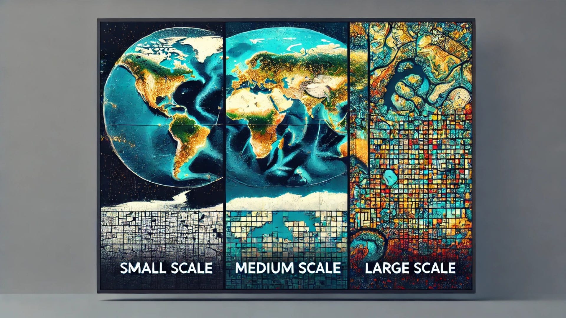
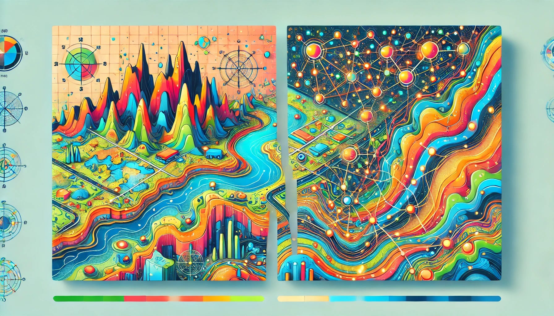
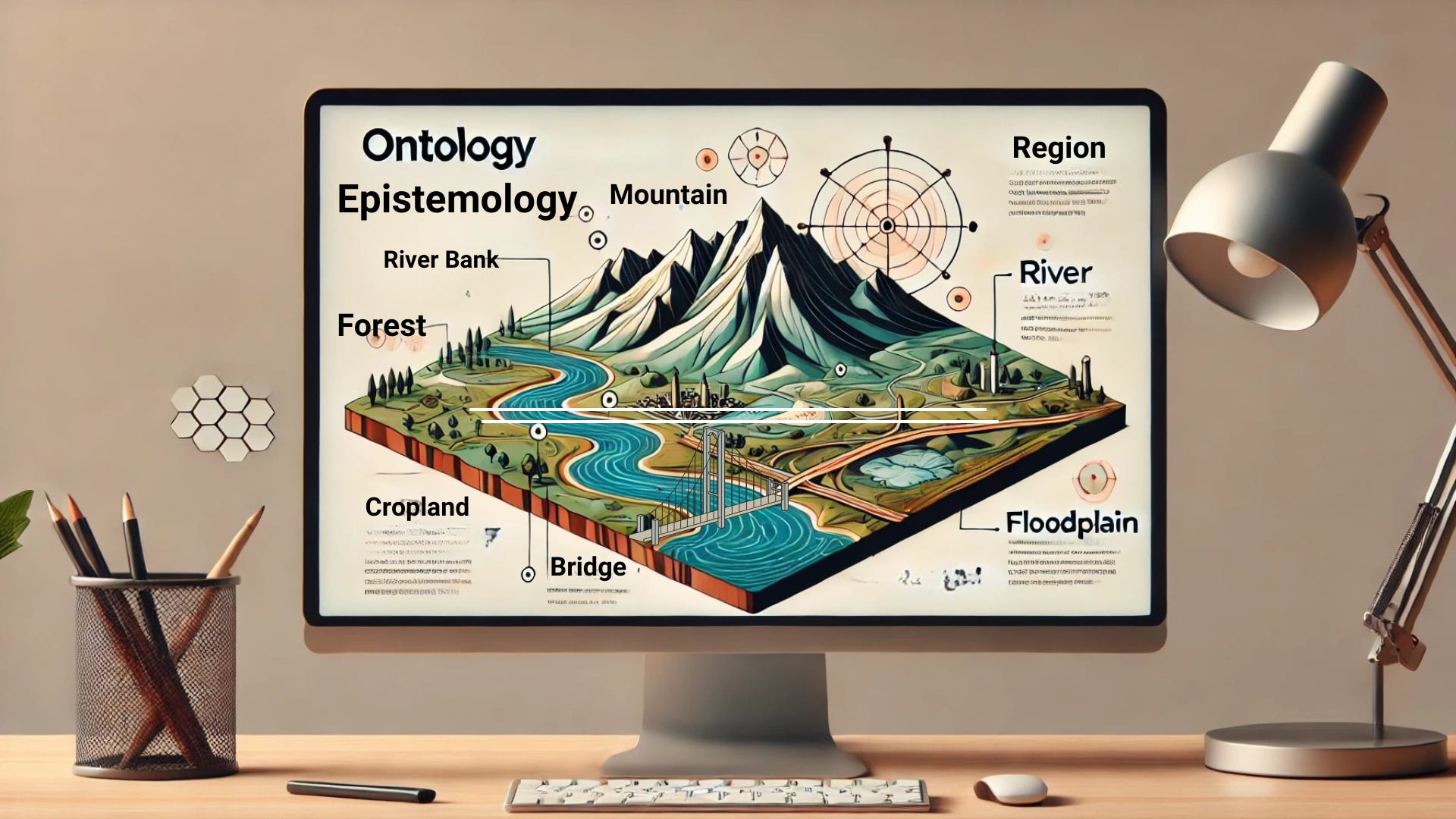
To make maps, we must sin against the landscape. We distort the earth’s roundness, and we simplify complex realities down to a series of colors and symbols. Ancient trees become a scattering of green pixels on a screen; a horrific battle becomes a labeled dot; and an awe-inspiring bird migration becomes a simple arrow.
But this is necessary. Maps work because they abstract and generalize (as noted by Arthur Robinson, who said “the act of generalization gives the map its raison d’être”). They help make reality comprehensible by packaging it into chunks that our brains can digest. However necessary, though, these generalizations are still sins, and maps can never be truly “accurate.”
It’s something I’ve struggled with throughout my career. How much should I generalize? I’ve talked about this in the past: If I smooth out a line representing a river, did I do it too much? Or not enough? Would someone else have done it differently?
No matter how much I fret, however, my...
GeoFeeds Daily Briefing — Sunday, July 19, 2026 Covering posts from 0800 ET July 18 to 0800 ET July 19. Sources: 162 geospatial feeds. Quiet day across the feeds. As is typical for a mid-summer weekend, the window ran nearly empty — the trade, vendor, and analyst feeds went dark, leaving mostly community and slice-of-life posts. The week's substantive news all landed Thursday through Saturday and was covered in prior briefings: the Esri User Conference wrap-up in San Diego, Cercana's twin weekly and Esri-UC supplemental briefings, the xyHt-reported Topcon–GreenValley LiDAR partnership, Metaspectral's Planet/Tanager hyperspectral tie-up, and EarthStuff's continuous-simulation flood-risk study. Against that, the day's backdrop was the 2026 World Cup final — which surfaced in the feeds only as a Mappery reader photo of a promotional cap. One recurring digest is worth a look. Highlight weeklyOSM 834 — weeklyOSM The OpenStreetMap community's weekly digest, covering July 9–15, posted...
Today is the final of the 2026 World Cup. Ken was very pleased to get this special baseball cap “These Adidas “World Cup” hats are promotional items. Chuffed to bits to have acquired one”
I am sure he will be wearing it to watch the game.
GeoFeeds Daily Briefing — Saturday, July 18, 2026 Covering posts from 0800 ET July 17 to 0800 ET July 18. Sources: 162 geospatial feeds. Three Topics That Stood Out 1. The Esri User Conference closes, and the verdict is "an AI system with a map inside it" The week's dominant story got its clearest editorial framing as the conference wrapped in San Diego. Cercana's supplemental briefing on the 2026 Esri UC argues that under the "GIS—Creating a more intelligent world" theme, Esri spent five days making one case repeatedly: ArcGIS is becoming an AI platform first and a mapping platform second. Independent coverage lines up — the conference drew more than 18,000 in-person attendees and Esri laid out a three-tier AI architecture (purpose-trained GeoAI models, embedded AI Assistants for plain-language workflows, and agentic AI that runs multi-step geospatial tasks), with MCP surfacing as the integration layer that lets any enterprise agent call ArcGIS on demand. Why this matters: This is...
Grégoire shared this Wall map in Nygården B&B (Harmånger, Sweden) about the neighbouring village of Nordanå.
He said it is maybe 6×3 meters and colorised. Quite nice!
NYCSim is a truly impressive digital twin for New York City. Part real-time spatial platform and part living sandbox, this browser-based simulator allows you to explore a virtual Manhattan from the comfort of your own home. By pulling in live municipal transit data, real-time air quality metrics, and local weather feeds, the platform transforms a static city plan into a living, breathing map.&
A VerySpatial PodcastShownotes – Episode 78912 July 2026
Some of our current questions
Click to directly download MP3
YouTube (audio only)
AVSP – Episode 789 Transcript (docx)
http://traffic.libsyn.com/avsp/AVSP_Episode789.mp3
Web corner
Destination Earth
Topic:
Questions we currently have about Geography/geospatial
Music:
Around You (Ft. Alyssa) by REYUS
Topcon Positioning Systems announced it has entered a strategic agreement with GreenValley International (GVI) to collaborate on technologies for surveying, mapping, construction, forestry and other spatial intelligence related applications. Planned innovations will include integrated hardware and software solutions for handheld, aerial, and mobile LiDAR data collection and processing workflows, with developments extending into robotic systems, autonomous monitoring solutions and real-time cloud-based data processing and transfer.
“Collaborating with GreenValley allows us to combine the strengths of both organizations and deliver simpler, more efficient workflows to more professionals,” said Ron Oberlander, head of the Topcon Geomatics and Construction Platforms. “By advancing joint research and integrating emerging AI technologies into spatial solutions, we aim to help users collect, process, and apply data more effectively, even in remote and challenging...
I am NOT associated with HR/recruiting in ANY wayTherefore, these are NOT endorsements, and there are no ‘referrals’ or the like for meI am simply sharing SOME roles that I have seen – in the hope that they are of use to someoneAs such, I am not (and indeed can not) in any way ‘vet’ these roles (i.e., PLEASE do your ‘due diligence’ / use your judgement (with the hideous prevalence of ‘ghost jobs’, ‘fishing’, fraudulent so-called recruiters, etc))Further, roles listed are in no specific order (i.e., simply as I ‘encountered’ them during the week)There is ZERO cost to access this list of spatial / GIS rolesI am not (really) ‘mining’ US Federal government roles - with the ‘hiring freeze’, uncertainty, etcYou can subscribe to (a) the (free) weekly LinkedIn newsletter www.linkedin.com/build-relation/newsletter-follow?entityUrn=7397678824928366594 or (b) also for free at earthstuff.substack.com - if so inclined#fridayjobs #gischat #jobsonfriday #GIS #spatial #mapping #cartography #geography...
If you use any of the GIS web services provided by the ITS Geospatial Services Bureau, you will need to update your connections in the coming months. They are migrating services to a new platform. As announced in May, the NYS Geocoder is now available on the new GeoHub platform (NYS Geocoding Service | gis). […]
In the spring of 2024, through the work of (now retired) Acquisition Specialist Robert Morris, the Geography & Map Division acquired a significant set of manuscript maps of the North American west coast created by the Spanish Hezeta-Bodega y Quadra Expedition of 1775. These maps, now known as the Bodega y Quadra 18th century coastal chart collection, 1775-1792 represent some of the earliest detailed European mapping of the North American west coast, ranging from the central Californian coast all the way up to Sitka, Alaska.
Image 11 of Bodega y Quadra 18th century coastal chart collection, showing a Spanish land claim to modern-day Trinity Bay in California. Geography & Map Division.
In order to full tell the story of these maps, the Geography & Map Division has just published “Charting America’s West Coast: How the Hezeta-Bodega y Quadra Expedition of 1775 introduced Europe to the middle latitudes of North America’s west coast.”
Screen capture from “Charting America’s West Coast.”...
A new job has been added to the NYS GIS Association website. Visit the GIS Job Postings page to view GIS jobs. The NYS GIS Association is your source for GIS jobs in NYS!
Spatialists – geospatial news
• By Ralph Straumann
•
The swisstopo app, downloaded more than four million times since 2020, gets three notable updates: 300 curated #landmarks now appear on the basemap with in-app photos and background info, #search works cross-lingually and even tolerates dialect and typos, and #route #planning has been overhauled with flexible start points, times, and elevation filters. A solid refresh for one of Switzerland’s most popular apps, used up to 300,000 times a day on sunny weekends.
FAA and EASA leaders take the stage together on the final day of Commercial UAV Expo 2026 for a candid comparison of transatlantic BVLOS regulation. Las Vegas, NV, USA — July 16, 2026 — Commercial UAV Expo, the world’s leading commercial drone trade show and conference, has announced its second and final keynote for the 2026 event: […]
Week of July 11–17, 2026. Published July 17, 2026. Sourced from the geofeeds ecosystem and open web reporting. Executive Summary The 2026 Esri User Conference, which closes today in San Diego, made one case over and over: ArcGIS is turning into an AI system with a map inside it. Under the theme “GIS—Creating a more […]
GeoFeeds Daily Briefing — Friday, July 17, 2026 Covering posts from 0800 ET July 16 to 0800 ET July 17. Sources: 162 geospatial feeds. Three Topics That Stood Out 1. Environmental change, mapped from the tundra to the coastline Within a single day, three feeds put land-surface change at the center. EarthStuff surfaced an open-access study that replaces single design-storm flood maps with 82 years of continuous simulation, finding that deterministic 10-year events underestimate flood depths by up to half a meter and that one meter of sea-level rise quintuples King County's expected annual flooded area (161 → 787 hectares). Spatial Source covered how historical maps are guiding Australia's 30% revegetation target, and Earth Observation News reported UAV vegetation surveys in Svalbard's Reindalen to study reindeer habitat. Different biomes, one throughline: watching how landscapes shift. Why this matters: Conservation and climate-resilience GIS stay structurally underserved in the...
162 feeds monitored. Published July 17, 2026. Executive Summary Trustworthy geospatial data moved closer to the center of the AI market this week. Overture Maps Foundation crossed 50 members and used the milestone to make a direct case for open, interoperable base data as grounding for AI systems. Geospatial foundation models also became more accessible. […]
Today in our OpenStreetMap (OSM) interview series we are speaking with Matthew Whilden about his journey as an OSM mapper, his work supporting the community through the OpenStreetMap US Board, and his passion for creative mapping. From parks and playgrounds to hidden features discovered through geocoding and aerial imagery, Matthew’s story highlights the curiosity and community spirit that shape OpenStreetMap.
Here is an example of the cathedrals of Germany that we created using Matthew’s XofY tool.
1. Can you introduce yourself and tell us a bit about your OpenStreetMap journey? What first got you hooked on mapping?
I started adding parks and playgrounds when my daughter was born. Both as a simple pastime while she napped, but also a way to explore more things to do with her as she got older. Editing the map is a lovely way to learn more about the world.
2. You’ve mentioned using geocoding to turn lists of addresses into mapping adventures, for example tracking down drive in...
This animated map reveals how agricultural productivity is expected to be affected by climate change around the world throughout this century. It uses the new Climate-Driven Agricultural Decline Index (CADI) to show where and how global heating is likely to alter crop-growing conditions.According to the Climate-Driven Agricultural Decline Index, more than 640 million people already live in
Animation 1: Mitschnitt der Lighthousemap [1] um Rostock
Was Schönes zum Wochenende oder im Urlaub: Falls Ihre gerade irgendwo an einer Küste seid, schaut nach Leuchttürmen (auch Leuchtfeuer oder Befeuerung) und dann gleich auch mal in die Karte der Leuchttürme, die Lighthousemap [1] vom Geo Team der Universität in Groningen. Ganz sicher findet Ihr auch „Euern“ Leuchtturm.
Die Daten stammen via Overpass-API mit der Anfrage nach allen Elementen mit einem „seamark:light:sequence“- oder „seamark:light:1:sequence“-Attribut. Diese werden dekodiert und mithilfe von Leaflet als farbige Kreise auf der Karte angezeigt. Außerdem wird versucht, die Attribute „seamark:light:range“ und „seamark:light:colour“ zu berücksichtigen. Den Code findet Ihr auf GitHub [2]. Falls Ihr „Euern“ Leuchtturm nicht findet, ergänzt ihn einfach im OpenStreetMap und schon ist er auch auf dieser Karte zu finden
Animation 2: Mitschnitt der Lighthousemap [1] um ganz Europa
[1] …...
28th Offshore China (Shenzhen) Convention 2026 (OC2026) was held in Shenzhen on June 16–17, themed Venture Deep Seas, Drive Industrial Upgrade: Accelerate High-Quality Offshore Energy & Equipment Development, with a parallel core agenda Foster Win-Win Collaboration & Build Resilient Industrial Ecosystem.
--https://doi.org/10.5194/nhess-26-3231-2026 <-- shared #openacess paper--[part of my old stomping ground as an engineering geologist]H/T “Flood maps are usually built from a single design storm. For King and Pierce Counties in the Pacific Northwest (USA), [the authors] tried the opposite - simulate 82 years of actual coastal and river conditions (plus 18 synthetic years) with SFINCS and let the statistics fall out cell by cell. That took about 5,400 yearly simulations and 194,000 CPU hours on USGS’s Hovenweep HPC. Worth it!The design-event shortcut turns out to hide a real hazard. A deterministic 10-year event underestimated flood depths by up to half a meter compared to the continuous runs.The bigger surprise [to the authors] was how one-sided the climate signal is. One metre of sea level rise takes King County’s expected annual flooded area from 161 --> 787 hectares, almost a factor of five. Changes in storminess over the same horizon barely register. And somewhere between 100 and...
Historical maps have been used to picture what’s needed for Australia to meet its 30% re-vegetation goal.
The post Mapping helps show Australia’s vegetation future appeared first on Spatial Source.
By Lynn Cai
China is a country spanning over 9.6 million sq km (3.7 million square miles) , making it one of the largest countries by landmass. The country is geographically diverse, with biomes and climates ranging from hot, arid deserts to the cold boreal forests.
Due to the country’s vast land area, subdividing it into regions is no easy task. The country is generally divided into six regions, covering the north, south, east, and west. The following categories include: North China, East China, Southwestern China, South Central China, Northeast China, and Northwestern China.
Highlighted on this map in dark blue, Northeast China is one of China’s coldest regions. Provinces in this region include Heilongjiang, Jilin, and Liaoning. Heilongjiang borders Russia, while Jilin and Liaoning share a border with North Korea. Major cities include Harbin, Changchun, and Shenyang. This region is mostly known for boreal and deciduous forests. North China, highlighted in green, consists of the...
How well do you know the town you call home? After twenty-six years in Denver, most of it tucked up in its northwest corner, I suspected my own honest answer would be “not very”. So when I decided to take a personal sabbatical of sorts this Spring to ponder a mid-career refactoring in the brave […]
The three northwestern coastal departments of Peru, Tumbes, Piura, and Lambayeque all voted solidly for the victorious rightwing candidate, Keiko Fujimori, in the 2026 election, giving her, respectively, 64.4%, 57%, and 58.9% of their votes. By Peruvian standards, these three departments are roughly average in terms of social and economic development (see the maps in the previous post). All three have agriculturally oriented economies, and all have long favored conservative, market-oriented policies.
One distinctive socio-cultural feature of northwestern Peru is its relatively large proportion of Afro-Peruvians. Black Peruvians constitute 11.5 percent of the population of Tumbes, 8.9 percent of the population of Piura, and 8.4 percent of the population of Lambayeque, the highest figures in the country. One might expect Afro-Peruvians to favor leftwing candidates, which is certainly the case in Colombia regarding Afro-Colombians (as can be seen on the final two maps posted below)....
Enrolments are open for the IBSC-recognised S-5B Hydrographic Surveyor and S-8B Marine Geospatial courses.
The post Hydrographic Surveyor, Marine Geospatial courses appeared first on Spatial Source.
The map above shows how many US Supreme court justices were born in each US State. The clear winner is New York with 14 followed by Virginia with 10.
Overall, there have been 116 justices since the Court was established in 1789.
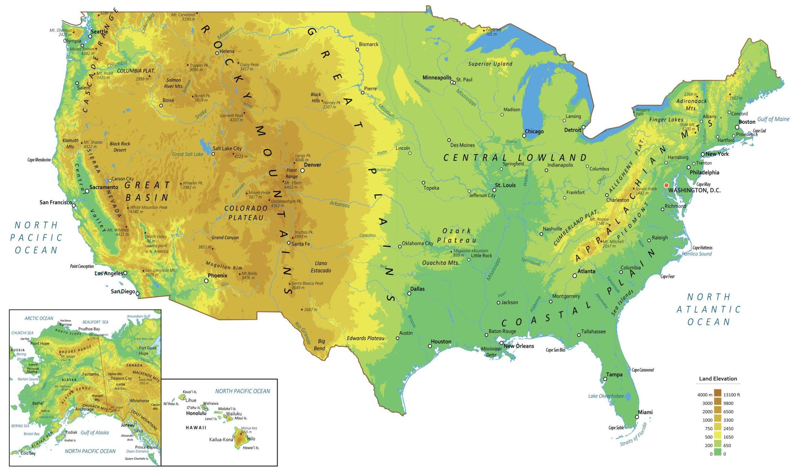
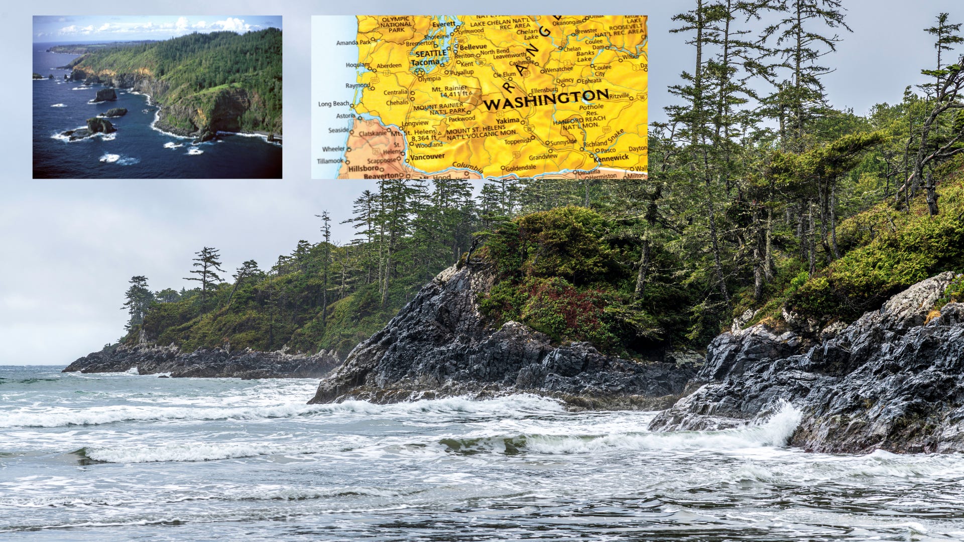
But, only 24 states have ever produced a justice, so more than half never have, including the entire Pacific Northwest, Florida, and almost everything between Kansas and California.
The centre of gravity has shifted dramatically: Virginia and Kentucky dominated the first century, New York dominates overall, and no justice born west of Colorado has ever served except the three Californians.
Here is a full list by state:
US Supreme Court Justices by Birth State
#scotus-birth-states {
font-family: Georgia, 'Times New Roman', serif;
max-width: 760px;
margin: 0 auto;
padding: 24px 16px;
color: #1f2933;
line-height: 1.6;
}
#scotus-birth-states .sbs-intro {
font-size: 1.05em;
margin-bottom: 28px;
}
#scotus-birth-states h2 {
font-size:...
Vancouver, B.C. — July 15, 2026 — Metaspectral announced its partnership with Planet Labs PBC, a leading provider of daily data and insights about change on Earth, to deliver trusted, evidence-based spectral intelligence from Planet Tanager™ hyperspectral data through Metaspectral Clarity. Planetary Intelligence derived from Planet data is emerging as a new model for understanding the physical world: continuous sensing, […]
Sigma Advanced Systems, the parent company of Nasmyth, has acquired UK aerospace manufacturer Bromford Precision Solutions in a strategic move that further strengthens Nasmyth's manufacturing capabilities and reinforces the Group's position within the global aerospace and defence supply chain.
GeoFeeds Daily Briefing — Thursday, July 16, 2026 Covering posts from 0800 ET July 15 to 0800 ET July 16. Sources: 113 geospatial feeds. Three Topics That Stood Out 1. Open and authoritative data positioned as the substrate for AI Overture Maps Foundation announced it has reached 50 members — nearly double its 2024 count — with new additions including Grab, Uber, Samsara, Fresno County, and UC Santa Cruz, framing the milestone explicitly around standardizing open spatial data and GERS identifiers "to ground AI." In parallel, Esri expanded its Community Maps Program so ArcGIS users can push real-time road closures directly into Google Maps and Waze, with more than 100 communities already contributing authoritative data. Both moves treat curated base data as the thing large downstream systems depend on. Why this matters: This is the Open Data Evolution thread turning practical. Overture's "ground AI" framing echoes its own "Billion-Dollar Data Trap" argument that open map data is...
Wijfi shared these pictures, saying: “Some children drew a huge map of the Anderston and Finnieston neighbourhoods in the west end of Glasgow. Maybe not 100% spatially accurate, but an interesting depiction of how a kid sees this area.”
Where is Downtown? is an interactive map surveying tool designed to crowdsource the boundaries of "downtown" for any city. The process is very simple:Enter the name of a city into the search barDraw your perceived outline of "downtown" on the mapView a heatmap of all the collective responses submitted so farIf you are only interested in exploring where others think downtown is, you can skip
The deal will connect RocketDNA’s drone survey data API directly into the Deswik.CAD mine model space.
The post Drone firm RocketDNA does deal with Deswick appeared first on Spatial Source.
Hyades, founded by three young university graduates, is building “end-to-end intelligence for spatial data”.
The post New Zealand AI spatial start-up raises $1.25m appeared first on Spatial Source.
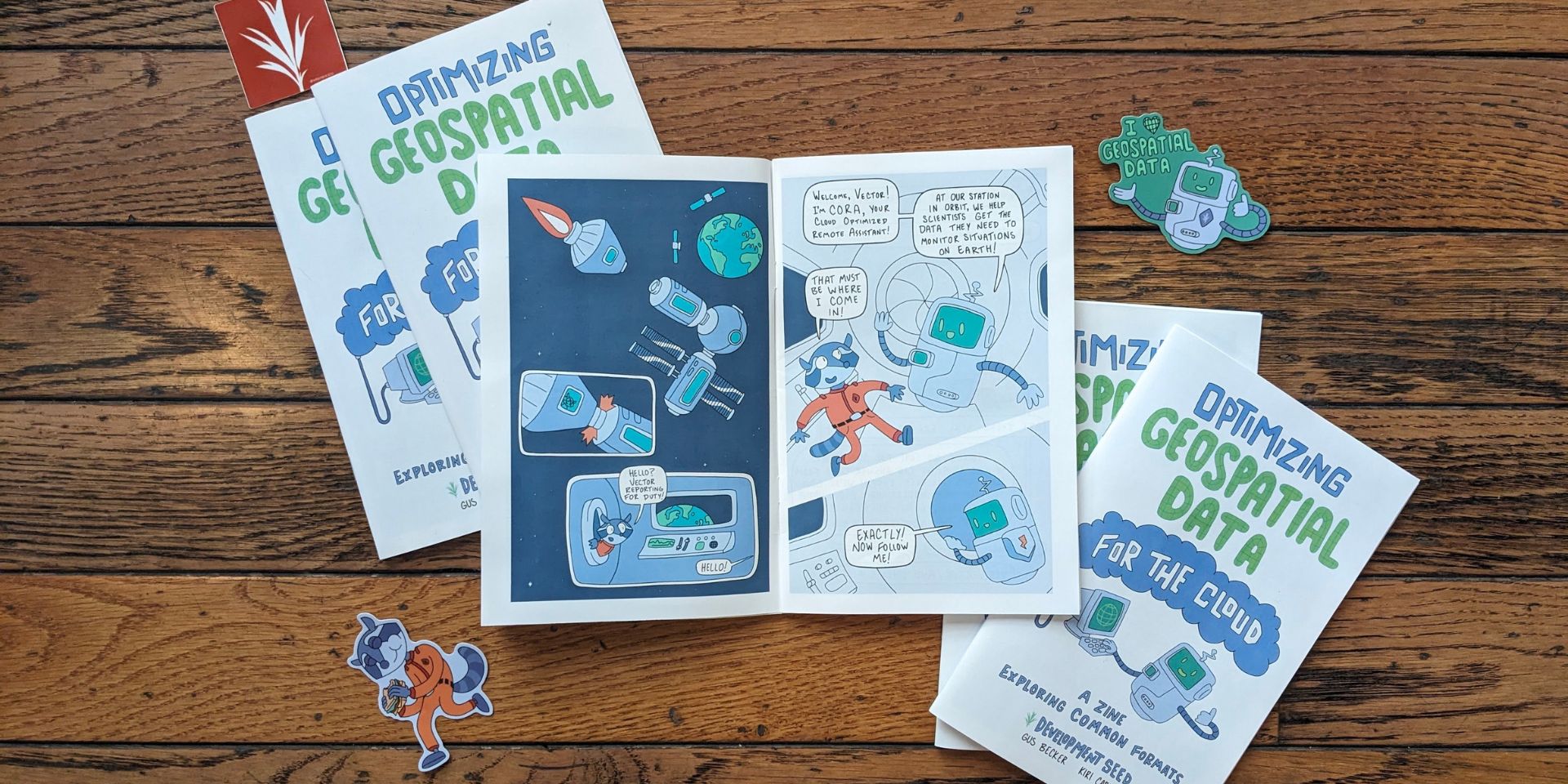
Wenn Ihr Euch schon immer mal einen Überblick über die Cloud-optimierten Geodatenformate verschaffen wolltet, dann seid Ihr im Blog-Eintrag meines Geo-Fachkollegen Mathias Gröbe von w12g [1] genau richtig. In seinem Beitrag „Geodaten in Cloud-optimierten Formaten in QGIS nutzen“ [2] beschreibt Mathias einfach und verständlich einige wesentliche technische Fakten sowie die verschiedenen Formate und deren Nutzung im freien QGIS. Folgende Formate werden im Beitrag vorgestellt:
Raster: Cloud-optimized GeoTIFF
Punktwolken: Cloud Optimized Point Cloud (COPC)
Vektordaten: FlatGeobuf
[1] … https://w12g.de/[2] … https://w12g.de/2026/geodaten-in-cloud-optimierten-formaten-in-qgis-nutzen/
Spatialists – geospatial news
• By Ralph Straumann
•
Konstantin Klemmer et al.’s #ISPRS 2026 tutorial on #FoundationModels and #EarthEmbeddings pairs free, MIT-licensed slides with hands-on Colab notebooks spanning four practical use cases, from direct #prediction to geo-#semanticSearch. Kiri Carini’s companion resource roundup rounds out the reading list for anyone diving into this fast-moving corner of #GeoAI.
The AGS Globe: Ancient Urbanism on the Mississippi: The Geography of Cahokia by American Geographical Society
The American Geographical Society’s Weekly Newsletter for Tuesday, July 14, 2026.
Read on Substack
Members spanning technology, public sector, academia and non-profits standardize on open spatial data and unique IDs via GERS Summary Overture’s membership has nearly doubled since 2024, with new additions spanning tech, government, academia, and non-profits (including Grab, Uber, Samsara, Fresno County, and UC Santa Cruz). By adopting Overture data across buildings, addresses, and administrative divisions, […]
New Titles Expand on Landmark Work to Showcase How GIS Drives Better Decisions Across Water and Land Management Esri will debut the Power of Where Collection at the 2026 Esri User Conference. The collection builds on the 2024 book The Power of Where by Jack Dangermond, extending its ideas into real-world GIS applications. New […]
GeoFeeds Daily Briefing — Wednesday, July 15, 2026 Covering posts from 0800 ET July 14 to 0800 ET July 15, 2026. Sources: 162 geospatial feeds. Three Topics That Stood Out 1. Esri spent a day wiring itself deeper into the enterprise stack Four announcements landed within hours of each other: ArcGIS for ServiceNow (covered by Geoconnexion), ArcGIS Velocity arriving on self-hosted ArcGIS Enterprise, and Nearmap becoming the exclusive aerial imagery provider for the Living Atlas (both via Earth Imaging Journal). HERE simultaneously launched its GIS Data Suite as-a-service, pitched explicitly at Esri users connecting "directly within ArcGIS environments." Why this matters: The dominant platform is becoming a distribution channel. Nearmap and HERE selling through ArcGIS, plus integration into ServiceNow's IT workflows, deepens the ecosystem's gravitational pull — data partners increasingly reach customers via Esri rather than around it. 2. Agentic GIS is producing deployment security...
Hey guys, here’s this week’s edition of the Spatial Edge — the GPT-5.6 Sol of geospatial news. We’re not as impressive as some other news outlets, but we’ll get you where you need to go… In any case, the aim is to make you a better geospatial data scientist in less than five minutes a week.In today’s newsletter:US Census: Harmonising 30 years of housing data.Green Growth: Satellites track cleaner economic growth.Africa’s Power: Mapping future electricity expansion.Methane Trends: Wetlands mask emission reductions.Earthquake Damage: Satellite dataset for building damage.Subscribe nowResearch you should know about1. Fixing the fragmented history of US census dataFor researchers trying to track long-term socioeconomic trends in the United States, the decennial census can be a pain... Every ten years, the census redrawing process updates the boundaries of ‘block groups’ to reflect population shifts and urban development. While this keeps current data accurate, it basically fractures the...
Countries of the World with No Borders: Minefield
Minefield Quiz
Countries of the World with No Borders
Every border on Earth has been erased. Click where each country is on the blank map. One wrong click and it all goes boom.
Find
–
Found 0/168
Time 0:00
Mines
+
–
Reset
Choose your mode
Sudden Death
One wrong click ends the game
Three Strikes
Three wrong clicks allowed
Zoom and drag to reach the small ones. The sea is safe. Wrong countries are not.
Boom.
Share your score
Copy
Facebook
X
Threads
Bluesky
...
Hi everyone,
I hope you are enjoying the summer.
Today we have a quick note to share that we’ve launched a visual refresh of
our GDPR / data protection page.
Specifically:
The page now has a table of contents for easier browsing.
We now explicitly list our third-party subprocessors in a table for easier scanning
We now explicitly list our data deletion schedule in a table for easier scanning
We now explicitly list the Technical & Organisational Measures (TOMs).
Clarified that geocoding queries are NEVER used for AI training.
As with all of our pages, it is now also available in Markdown format (via the “Copy Page” toggle at the top of the content, or appending .makrdownto the URL
The Change History of the page was getting a bit long (GDPR took effect more than seven years ago!) so it is now hidden behind a clickable toggle.
Just to be clear: there has been absolutely no change in our commitment to and...
Building a place based data trust for people and planet
• By Leslie Hodge
•
Leslie Jasen Hodge took over as the Director of the Anguilla Department of Lands and Surveys (DLS) in 2014 with the goal of modernizing land administration island-wide. A limited government budget meant that many of his initially envisioned reforms were not immediately possible, however significant damage to the DLS building by Hurricane Irma in 2017 […]
Im QGIS-Plugin „GeoBasis_Loader“ [1] sind seit der letzten Meldung einige neue Themen hinzu gekommen, z. B. die Hochwasserdaten für Sachsen, Feldblockdaten für Brandenburg und Sachsen-Anhalt und Themen des DWD. Damit sind jetzt 856 Themen verfügbar, die aktuellen Änderungen findet Ihr wie immer unter Meldungen & Störungen [2] und Status [3].
[1] … https://geobasisloader.de/[2] … https://geoobserver.de/gbl-aktuelle-meldungen-stoerungen/[3] … https://geoobserver.de/qgis-plugin-geobasis-loader/#jsonstatus
Last month I posted a review of Klimadashboard's European Heat Tracker, which visualizes how many people across Europe are exposed to extreme heat in real time. Since then, temperatures have continued to exceed seasonal norms across much of the continent, and new mapped visualizations have continued to document the unfolding heatwaves.
El País' How Extreme is this Heat? uses a
HawkEye 360, the global provider of signals intelligence data and analytics, announced that a model of its original Pathfinder satellite is now featured in the Smithsonian’s National Air and Space Museum on the National Mall within the newly opened RTX Living in the Space Age Hall.
Esri is launching ArcGIS for ServiceNow, an integration that connects ServiceNow, the AI control tower for business reinvention, with ArcGIS, bringing location intelligence into everyday enterprise workflows.
--The AGS GlobeThe AGS Globe: Ancient Urbanism on the Mississippi: The Geography of CahokiaRead more7 days ago · 19 likes ^^^^ shared technical article--https://doi.org/10.3389/frsc.2019.00006 <-- shared paper--https://libarts.source.colostate.edu/north-americas-first-city-20000-people-in-1050-c-e/ <-- shared technical article--https://www.nationalgeographic.com/science/article/131030-cahokia-native-american-flood-mystery-archaeology-pollen <-- shared technical media article--https://en.wikipedia.org/wiki/Cahokia <-- shared wiki page--H/T “When people think of pre-Columbian cities in the Americas before European colonization, examples such as Tenochtitlan, Chichen Itza, or Cusco usually come to mind. However, few know that there is another pre-Columbian city located in the present-day United States: Cahokia. Known for its impressive mounds, Cahokia in the 12th century CE was the largest metropolitan area and the most complex political system in North America north of Mexico.Cahokia...
--https://doi.org/10.1016/j.envc.2026.101568 <-- shared paper--H/T @Pollob Chandra Talukder“Deforestation poses a growing threat to biodiversity, ecosystem services, and sustainable development in Bangladesh, particularly in Gazipur, home to approximately 86% of the country’s Sal (Shorea robusta) forest. To identify future deforestation hotspots, we developed a machine learning-based framework integrating 12 biophysical, landscape, and anthropogenic conditioning factors with five machine learning algorithms (RF, XGBoost, ANN, NB, and MLP). Random Forest achieved the highest predictive performance (Accuracy = 84%; AUC = 0.93), followed by XGBoost (Accuracy = 83%; AUC = 0.92). The analysis identified rainfall and population density as the dominant drivers of deforestation, while probability maps highlighted the south-western and north-eastern parts of Gazipur as the most vulnerable. The findings provide a scientific basis for evidence-based forest governance, land-use planning,...
Spatialists – geospatial news
• By Ralph Straumann
•
#GeoLibre reached version 2.0 (and, a day later, 2.1): A browser-based, #cloudNative GIS that bundles vector and raster tools, a #CesiumJS 3D globe view, #DuckDB-backed spatial #SQL, and a natural-language assistant. Developed by Qiusheng Wu and contributors, GeoLibre also runs as a desktop app, on Android, and embedded in #Jupyter.
Voronoi diagrams answer one of the oldest questions in spatial analysis: for any location, which of my points is closest? Draw the boundaries where “closest” flips from one point to another and you get a honeycomb of polygons — one per point, jointly covering the whole plane. Hydrologists call them Thiessen polygons and have used them to weight rain-gauge data for over a century; the same construction underpins service-area estimation, school catchments, retail trade areas and nearest-facility analysis.
Generating one from your own points
You don’t need PostGIS or a QGIS processing chain for this. Upload a point layer — GeoJSON, shapefile, KML, GeoPackage, or a CSV with coordinates — to this Voronoi diagram generator and it computes the polygons in your browser and exports them in any of the same formats. Each polygon carries the attributes of its seed point, so a join is unnecessary — the store’s sales figures are already on its trade-area polygon.
Two practical settings matter:
The...
UTM coordinates look reassuringly precise — 630084 E, 4833438 N — right up until someone asks you to put them on a web map, which speaks latitude and longitude. Then you discover the two facts that define every UTM conversion: the numbers are meaningless without a zone, and ambiguous without a hemisphere.
The 60-zone problem
UTM divides the world into 60 north–south strips, each 6° of longitude wide, and restarts its easting count in every one. That same 630084, 4833438 pair exists in all 60 zones — in zone 18 it’s on the US East Coast; in zone 30 it’s in Spain. If a dataset arrives as bare UTM coordinates with no zone in the metadata, the zone has to come from context (the .prj file, the data provider’s docs, or knowing roughly where the data should be).
The classic failure mode is subtler: southern-hemisphere data without the hemisphere flag. Southern UTM northings are offset by 10,000,000 m; forget the flag and your Australian survey points land in the North Pacific.
Converting a...
Few things cause quieter data bugs than direction conventions. A surveyor’s field notes, a navigation app, and a Turf.js calculation can all describe the same direction with three different numbers — and if you mix them without converting, everything still runs, it’s just wrong.
The three conventions you’ll actually meet
Azimuth (0–360°): measured clockwise from north. East is 90°, south is 180°, west is 270°. The standard in surveying, artillery, astronomy and most navigation instruments.
Signed bearing (-180° to +180°): positive east of north, negative west of north. South is ±180°, west is -90°. This is what Turf.js, PostGIS’s ST_Azimuth-derived workflows and many GIS libraries return — which surprises people expecting compass values.
Quadrant bearing (N 45° E): the classic surveyor’s notation — an angle up to 90° referenced from north or south, toward east or west. Still standard on legal descriptions and older survey plats.
Converting between them
The azimuth signed-bearing...
OpenStreetMap is the largest open geographic database in existence, but “download some of it” is famously non-obvious. The full planet file is over 80 GB, the export tab on openstreetmap.org caps out at a few thousand nodes, and Overpass QL has a learning curve that stops most people at the first curly brace.
What most GIS work actually needs is simpler: the buildings, roads or points of interest for one town or study area, in a format QGIS or a web map can open. Here are the practical routes, from easiest to most powerful.
1. Browser extraction for a drawn area
The fastest path for small-to-medium areas: draw a bounding box, pick a theme, and download OpenStreetMap data as GeoJSON, shapefile, KML or GeoPackage directly from your browser. The tool queries the Overpass API for you — no query language required — and converts the result client-side. Good for anything up to a city-sized extract of a single theme (all buildings, all highways, all amenities).
2. Geofabrik for country and...
GeoTIFF is the workhorse raster format of GIS: elevation models, satellite imagery, drone orthomosaics and scanned historical maps all ship as .tif files with embedded georeferencing. The catch is that double-clicking one opens a photo viewer that either refuses to load it or shows a black rectangle — because photo viewers know nothing about 16-bit elevation bands or geographic coordinates.
Viewing a GeoTIFF without desktop GIS
Drop your file into this free online GeoTIFF viewer and it renders the raster on an interactive map, reads the embedded coordinate system, and reports the metadata that matters: band count, data type, pixel resolution, extent and CRS. Processing happens client-side in your browser with GDAL compiled to WebAssembly — the file never leaves your machine, which matters when the imagery is client data.
Why your GeoTIFF looks black (or white)
The most common GeoTIFF confusion isn’t opening the file — it’s opening it successfully and seeing nothing. This is almost...
The shapefile has been declared dead more times than any format in GIS, and yet it remains the default way spatial data gets handed around. Sooner or later someone emails you a ZIP full of .shp, .dbf and .prj files and just wants to know: what is in this thing?
Installing QGIS or requesting an ArcGIS license is overkill for that question. Browser-based viewers can now parse a shapefile locally — the file never leaves your machine — and render it on an interactive map in seconds.
The quickest option: a browser-based shapefile viewer
Upload your zipped shapefile to this free online shapefile viewer and it renders the geometry on a map with a full attribute table. It runs entirely client-side (the processing happens in your browser via WebAssembly), so it works with sensitive data too — nothing is uploaded to a server.
A few things to check before you upload:
Zip the whole set. A shapefile is not one file — at minimum the viewer needs the .shp (geometry), .dbf (attributes) and .shx...
FME Blog - FME by Safe Software
• By Tiana Warner
•
Key takeaways:
Exposing an FME workspace as a callable MCP tool gives any client FME’s full capabilities rather than raw access to your databases and file systems.
The safest place to filter data is at the source: strip or never load sensitive attributes so they can’t be returned by accident.
Running the model, client, and server entirely on-premises keeps sensitive data behind the firewall.
You don’t need frontier models for everything: matching a smaller local model to a well-scoped task controls cost and keeps processing and data inside your network.
Tool, server, and parameter descriptions are what let a model pick the right tool, so treat documentation as part of the build, not an afterthought.
Modern enterprises want to put AI to work on valuable data that lives in on-premises databases, file shares, CAD and BIM repositories, geospatial systems, and more. But of course, it’s unwise to give AI direct access to production data and systems....
This penultimate post on the 2026 Peruvian presidential election examines the relationship between the electoral results and socio-economic development at the departmental level. Not surprisingly, the rightwing candidate Keiko Fujimori generally supported the interests of the business community and the wealthier segments of society, whereas the leftwing candidate Roberto Sánchez focused more on marginalized communities and the poorer segments of society. One might therefore expect Fujimori to have done better in Peru’s more economically productive departments, as reflected by per capita GDP figures. But as it turned out, departmental GDP per capita was a poor predictor of election results. As can be seen on the paired maps posted below, Sánchez won the most economically productive department, Moquegua, as well as many of those in the second-highest tier. He also won the lowest-ranked department, San Martin, and many of those in the second-lowest tier. By the same token, Fujimori took...
Welcome to the 146th issue of Geospatial Jobs, a newsletter focusing on data science and geosciences (🌧climate-tech, 🌽ag-tech, 🌊risk modeling, ⚡️energy, 🛰remote sensing, ♻️sustainability, and more).The paywall on issue #142 is removed and it’s now freely accessible. Shout out to Manjaree Binjolkar and Apoorva Shastry who voluntarily helped with formatting this issue.Share🕵️💵 Recent Fundraisings / Updates:Adaptive Insurance raised $5M to expand specialty insurance products for climate resilience.💡📚 Useful Resources:ECMWF released earthkit version 1.0, providing a flexible set of tools for accessing, processing, analysing and visualising meteorological and climate data.Microsoft Research AI for Science released Aurora 1.5, the richer and more detailed open weather and climate model.USDA Joint Fire Science Program‘s FY2027 Notice of Funding Opportunity (~ $9M).PhD positions:Kansas State U: ML & remote sensing for water resources and wetland systemsUIUC: GeoAI & socio-spatial data...
How Much of America Have You Seen?
Road Trip Log
How Much of America Have You Seen?
Tick off every US state you have set foot in, and see what share of the country you have covered by states, land area, population and GDP.
Click states on the map to mark them visited, or use the list below.
Clear all
Your coverage
0 of 0 states
Share your score
Copy
Facebook
X
Threads
Bluesky
LinkedIn
Copied to clipboard
Figures use approximate 2024-25 estimates for total area, population and nominal GDP. Percentages are shares of the totals of all 50 states (District of Columbia not included).
...
US States with No Outlines: Minefield
Minefield Quiz
US States with No Outlines
The borders are gone. Click where each state is on the blank map. One wrong click and it all goes boom.
Find
–
Found 0/50
Time 0:00
Mines
Choose your mode
Sudden Death
One wrong click ends the game
Three Strikes
Three wrong clicks allowed
Clicking the sea is safe. Clicking the wrong state is not.
Boom.
Share your score
Copy
Facebook
X
Threads
Bluesky
LinkedIn
Copied to clipboard
Play again
Alaska and Hawaii are down there on...
How Much of the World Have You Seen?
Expedition Log
How Much of the World Have You Seen?
Tick off every country you have set foot in, and see what share of the planet you have covered by countries, land area, population and GDP.
Click countries on the map to mark them visited, or use the list below. Micro-states and small islands are in the list.
Clear all
Your coverage
0 of 0 countries
Share your score
Copy
Facebook
X
Threads
Bluesky
LinkedIn
Copied to clipboard
Figures use approximate 2024-25 estimates for land area, population and nominal GDP. Percentages are shares of the totals of all 197 countries...
Field crews have always run infrastructure using software built for something else. Field Operations Management (FOM) names the missing category: running, recording, and closing out physical field work. This post covers the category, why existing tools fall short, and why Fulcrum is a Field Operations Management platform purpose-built for the field.
Key insights
Field crews have run infrastructure for decades using software built for other jobs, with no category of their own.
Field Operations Management names that gap: running, recording, and closing out physical field work.
Customer service platforms, GIS systems, and construction apps each cover one piece of the work and drop it at the edges.
A completed asset can sit unclosed for months after construction ends, earning no return the whole time.
Records scattered across separate systems force crews to redo work that already exists somewhere else.
Fulcrum is a Field Operations Management platform, built to run...
GeoFeeds Daily Briefing — Tuesday, July 14, 2026 Covering posts from 0800 ET July 13 to 0800 ET July 14. Sources: 162 geospatial feeds. Three Topics That Stood Out 1. The Public EO Commons Frays While Commercial EO Buys Trust Spatialists surfaced Aravind Ravichandran's argument that Switzerland's decision to sit out Copernicus is a symptom rather than an incident: shrinking budgets, wavering political consensus, and commercial pivots are eroding Earth observation as a public good, and he floats an "EO Accord" modelled on past coordination successes. Hours earlier, EarthDaily published its answer to the same problem from the other side — announcing CEOS-ARD compliance, the first commercial optical constellation to claim it, ahead of data availability around September 2026, with the argument that provenance now matters as much as resolution. TerraWatch's own EO Essentials, meanwhile, logged China's CGSTL raising $736M largely from provincial governments and state-backed funds. Why...
The map above compares the Manhattan neighbourhood of Harlem with the Dutch city of Haarlem which it was named after. Surprisingly the two have very similar populations and median incomes as the table below shows:
Harlem (New York)Haarlem (Netherlands)
Population197,052162,543
Area3.63 km2
(1.4 sq mi)32.09 km2
(12.39 sq mi)
Density54,284/km2
(140,590/sq mi)5,572/km2
(14,430/sq mi)
Median Income$52,708 (€46,243)$49,589 (€43,500)
More general comparisons:
Harlem, New YorkHaarlem, Netherlands
TypeNeighbourhood within New York CityIndependent city and municipality
OriginsEstablished by Dutch colonists in the late 1650s as Nieuw HaarlemMedieval settlement granted city rights in 1245
SettingNorthern Manhattan, beside the Harlem RiverOn the River Spaarne, near Amsterdam and the North Sea
Best known forAfrican-American history, jazz, literature and the Harlem RenaissanceDutch Golden Age art, canals, historic architecture and...
En esta entrada de nuestro blog vamos a comentarte las mejoras y novedades más destacadas de la nueva versión de QGIS, la 4.2 que lleva como nombre Belém Do Pará. QGIS 4.2, se basa en la sólida base de la versión 4.0, la cual migró el núcleo de QGIS al marco Qt6. Esta versión añade nuevas ...
Leer más
QGIS 4.2, una versión marcada por la evolución en el modelado 3D
Esri announces that ArcGIS Velocity is now available for ArcGIS Enterprise, enabling real-time data analytics and automated actions in self-hosted environments.
TripGeo Air is an impressive new browser-based flight simulator that lets you fly over a photorealistic 3D model of the real world.What makes TripGeo Air particularly fun - besides the thrill of flying over your favorite landmarks - is the game's progression tasks. New pilots begin with simple circuit training before unlocking a series of paid jobs, including sightseeing flights, cargo
Symbolfoto (Bildquelle: Chris Gallagher auf Unsplash)
Das Hochwasser im Ahrtal ist nun genau fünf Jahre her und wir werden durch entsprechende Beiträge in der Medien wieder mal daran erinnert. Auch daran, sich mehr um die Hochwasser- und Katastrophenschutz-Problematik zu kümmern, am besten jeder in seinem Bereich, zeitnah. Der gestrige Beitrag in der ARD „Allein in der Flut“ [1] hat da was mit mir gemacht, schwer verdaulicher, sehr persönlicher Stoff, der uns auch vor Augen führt, dass vieles vermeidbar war. Und es stellt sich sofort wieder die Frage: Sind wir heute auch genügend vorbereitet?
Für mich der Anlass, gleich mal zu schauen, welche Daten zu Hochwasser-Gefährdung derzeit im Geobasis_Loader [2] verfügbar sind. Und, es sind tatsächlich nicht sehr viele. Neben den HQ200, HQ100 und HQ10 in Sachsen-Anhalt steht nur noch die Starkregenkarte zur Verfügung, eigentlich bundesweit, aber leider sind noch nicht alle Bundesländer mit ihren Daten integriert.
Und weil der Status...
--https://doi.org/10.1038/s43247-026-03515-x <-- shared paper--H/T @Peter Potapov | Researcher at the World Resources Institute (WRI)“This paper is] a strong example of multifunctionality analysis applied to conservation planning. The study mapped six ecosystem functions, including carbon storage, nutrient availability, water regulation, erosion control, habitat quality, and ecological connectivity. [The author] combined satellite data, field soil sampling, and spatial modeling for this comprehensive analysis.Two findings stand out.Old-growth forests had the highest multifunctionality index of any land cover type.78.5% of the top multifunctionality hotspots fall outside the region’s protected areas, even though PAs already cover more than 54% of the territory.Together, these results make a clear case for expanding conservation of the remaining Intact Forest Landscapes and primary forests in Patagonia and elsewhere…”--“Remote forest landscapes provide critical references for...
--https://brilliantmaps.com/third-rome/ <-- shared technical / history article--https://en.wikipedia.org/wiki/Succession_of_the_Roman_Empire <-- shared Third Rome wiki page--“The [first] map… shows which countries have claimed to the the successor to the Roman Empire at some point in their history (so called Third Rome). Learn more about each [in this article]…”#ThirdRome #RomanEmpire #Rome #successor #map #mapping #spatial #empire #civilisation #turkey #russia #byzantine #bulguria #serbia #greece #germany #austria #france #italy #history #ancienthistory #historiography #BrillantMaps
--https://doi.org/10.21203/rs.3.rs-10085674/v1 <-- shared paper--https://zenodo.org/records/17627111 <-- shared open data--H/T @Kyle Davis | Associate Professor at University of Delaware“Which fields are irrigated across the world’s cropland? [The author’s] new global high-resolution (30 metre) map of the world’s irrigated area is out now, and can answer just that![They] have just published [their paper (1st link above)] and the beta version of [their] global maps [2nd link above] for field-scale irrigated areas across the planet for the year 2024! This was produced with an unprecedented training set of nearly 400,000 ground truth points!...”--“Irrigation plays a critical role in global food production and climate adaptation and exercises profound influence over humanity’s water use. Yet despite its critical importance, there is a persistent lack of understanding of fine-scale irrigation patterns across the planet, knowledge which is essential for informing global food security and...
--https://www.theguardian.com/world/2025/feb/11/beavers-save-czech-taxpayers-by-flooding-ex-army-training-site <-- shared technical media article--https://en.wikipedia.org/wiki/Beaver-engineered_dam_in_the_Czech_Republic <-- shared wiki technical page--https://phys.org/news/2025-02-fine-beavers-czech-treasury-million.html <-- shared technical article-- ^^^^ shared video (Czech)--H/T @ScienceGirl“We don’t expect any conflict with the beaver in the next 10 years,” ~ Bohumil Fiser from the Czech Nature Conservation Agency--“For seven years, planners struggled to complete a $1.2 million wetland restoration project in the Brdy region of the Czech Republic. The goal was to build a dam that would improve water management and bring back valuable wetland habitat, but the project remained trapped in a maze of permits and approvals.Then a family of eight Eurasian beavers did what engineers had planned… without permits, machinery, or a budget.The beavers built a network of dams in almost the...
--https://noaaresearch.webex.com/wbxmjs/joinservice/sites/noaaresearch/meeting/download/9b3e684d45ca47fc9469070eabd9a142?MTID=m2fa4a8af7bd8647fc48619af5eeecb5a <-- shared NOAA Summer Science Series individual webinar--https://www.drought.gov/what-is-drought/flash-drought <-- shared NOAA overview technical article--https://www.star.nesdis.noaa.gov/star/NOAAScienceSeminars.php <-- subscribe to the NOAA Summer Science Series--https://doi.org/10.1038/s41612-024-00618-0 <-- shared paper--https://communities.springernature.com/posts/the-prevalent-life-cycle-of-agricultural-flash-droughts <-- shared technical article (derived from paper above)H/T Flash floods? not TOO hard to conceptualiseFlash drought? harder to ‘get my head around’, but H/T / presenter does/did an excellent job!“Not all droughts are the same. In some cases, drought rapidly intensifies at subseasonal to seasonal scales with significant impacts to agriculture and water resources along with the increased propensity for...
Map found via reddit, click for larger version
While it’s well known that the mercator projection distorts the world, the maps here show very clearly by how much. Countries close to the equator barely change, whereas countries further north shrink dramatically.
The maps are all the work of climate data scientist @neilrkaye.
You can see an animation below:
Map found via reddit, click for larger version
The map also gives a bar graph to show the relative size of the world’s largest countries:
New True Size Comparison Tool
#bm-truesize-root { all: initial; display: block; font-family: 'Source Sans 3', Arial, sans-serif; color: #1c2b45; background: #faf6ec; border: 1px solid #d8cdb4; border-radius: 10px; overflow: hidden; max-width: 860px; margin: 0 auto; line-height: 1.5; }
#bm-truesize-root * { box-sizing: border-box; }
#bm-truesize-root .bmts-header { background: #0f1c31; color: #f3ecdd; padding: 26px 28px 22px; position:...
What colors does the Earth actually come in? We built Sentinel-2 Paint to find out: a script that scours the Sentinel-2 archive for patches of every color the planet shows, and a browser app for playing with the results. Upload a photo and the app rebuilds it as a mosaic of real satellite imagery, nearest color per cell; pick a color and it shows the chip of Earth whose average color is closest, then flies to the exact scene and lat/lon where Sentinel-2 observed it. The idea is in the same spirit as NASA’s fun Your Name in Landsat tool, which spells out your name using Earth features shaped like letters — we do the same trick with color instead of shape. The palette behind the live app comes from 368 scenes and contains 92,916 unique Earth colors so far — about 0.55% of the 16.7 million colors in the 8-bit RGB cube. All the code is at github.com/calebrob6/sentinel2-paint.
A picture of one of the Sentinel-2 satellites, recreated by Sentinel-2 Paint (i.e. rebuilt entirely from...
Spatialists – geospatial news
• By Ralph Straumann
•
Switzerland’s decision to stay out of #Copernicus might be a symptom of a bigger problem, argues Aravind Ravichandran in the #Terrawatch Newsletter: shrinking budgets, wavering political consensus, and commercial pivots are chipping away at #EarthObservation as a public good. Aravind diagnoses the fragility of today’s #EO commons and proposes a possible fix, an “EO Accord” built on past coordination successes. #remoteSensing #Sentinel #Landsat
RCGS returns to Quest and Terra Nova with digital mapping technology University of Victoria’s MARMOTSat begins its mission in orbit Belleville reviews GIS practices after accidental data exposure GNSS resilience moves from a technical issue [...]
The post Geospatial Digest – July 13 2026 appeared first on GoGeomatics.
Latest vGIS News and Blogs
• By vGIS Support Team
•
A Fresh New Look Is Coming to vSite
Our latest biweekly release introduces a refreshed experience across vSite, with more intuitive navigation, redesigned pages, and new tools to make managing projects easier.
While the platform will have a modern new look, the functionality and workflows you rely on remain the same.
What’s Changing in vSite Web?
The updated interface organizes your workspace into three clear areas:
Project Data: View and manage 3D models, LiDAR scans, PDFs, redlines, and other project assets.
Projects & Settings: Switch between projects and manage preferences such as language, scan quality, image size, and units of measurement.
Map Tools: Access measurement tools, bookmarked views, cross-sections, map settings, and more.
Did You Know? You can use your Cost Codes to track quantities and redlines in vSite.
Release Updates
Portal
Redesigned My Profile and Projects pages
Redlines added to Project Dashboard analytics (Redlines...
FOSS4G NA - News - FOSS4G North America
• By Linda Stevens
•
The Call for Proposals for talks at FOSS4G North America 2026 will close Wednesday, July 15, 2026. This is your last chance to submit a talk proposal for this year’s program.FOSS4G North America 2026 will take place November 2–4 in Sacramento, California, and has already shaped up to include a strong mix of talks covering open geospatial tools, data, workflows, and real-world applications.As a reminder, after reviewing the first round of submissions, we had identified a few areas where we would still like to strengthen the program. We are especially encouraging additional talk submissions in the following areas:Business of Open SourceWe would love to see more talks focused on the business, sustainability, governance, and funding models that support open source geospatial work. This could include consulting models, product and service businesses, nonprofit and foundation support, public-sector investment, project governance, contributor pathways, or lessons learned from building and...
Every contractor knows utility strikes are expensive. Most assume the repair invoice is the number that matters. It isn’t, and the gap between what contractors expect to pay and what they actually pay is where projects, and sometimes companies, get into trouble.
The Scale of the Problem
US crews damage underground utilities an estimated 400,000 to 800,000 times per year — roughly one to two strikes every minute. According to the CGA’s DIRT Report, the CGA Index, which tracks year-over-year damage trends, rose from 94.0 in 2023 to 96.7 in 2024, signaling the industry is moving in the wrong direction. The total cost to the US economy is an estimated $30 billion annually.
What a Strike Actually Costs: Direct vs. Indirect
The direct costs are what most people think of: the repair crew, the materials, the emergency response. These are real. They are also, as the data shows, the smallest part of the bill.
Research examining utility strike incidents found that indirect...
Submitted by Evgeny, who simply says:
The new map of Izmir rapid transit I designed has been adopted as official one.
Transit Maps says:
Congratulations on this lovely little diagram becoming “official,” Evgeny!
There’s a lot to like about it, especially the intelligent use of a 30-degree grid to match the real-world geography of İzmir nicely, which also helps in setting all the labels horizontally without them running into each other. I also really like the subtle outline for the under-construction M2 metro line, which also shows that the diagram is future-proofed.
The diagram has to deal with two different scales: a relatively-compact urban area served by the Metro, trams and ferries, and the İZBAN suburban lines heading a long way north and south. Evgeny has dealt with this quite deftly, with the suburban lines outside the main area just being compressed substantially, with a minimum of space between the stations: I think this works quite well.
I also...
It’s time to kick off the longest running Map Calendar in History….probably.
We are looking for 14 or so so submissions for the calendar. I think last year we had a few more. We have judges randomly picked from out long sorted history that help us dig through and rate the submissions.
You can read up here on what we are looking for!
Your submission should be a map! Submit images please, (they’ll be printed after all), hi-res JPG or PNG, landscape orientation, 8 inches × 10.5 inches (20.32 cm × 26.67 cm) or proportional. See the sample below.
Please note that we may opt to place a semi-transparent box containing author information (Name and/or handle), the GeoHipster logo, and, potentially, a calendar sponsor logo. Please consider this, as well as about 1/4″ for bleed and 1/2″ for margins in your map design. If you have a preference as to which corner the box should be placed in, please note that at the time of submission.
While we want your map to be understood,...
Welcome to a new edition of Earth Observation Essentials, the free biweekly newsletter from TerraWatch covering key highlights from the EO market along with exclusive insights and analysis.If you would like a more detailed, comprehensive market briefing with exclusive analysis, delivered every week, become a Pro subscriber, or a Premium subscriber, for more deep dives on EO markets, technologies and applications.Upgrade
📈 EO Market Highlights
Major developments in EO
🛰 NASA’s cheapest missions deliver less scientific bang for the buck, a study from the Planetary Society found. This might probably be not true for EO given the success of NASA missions like TROPICS and CYGNSS among others.🇨🇳 Chinese satellite manufacturer Changguang Satellite Technology Co Ltd (CGSTL) raised $736M in funding from investors that included mainly provincial governments and state-backed funds. CGSTL which has about 161 satellites launched so far, said that the new round of financing will be to...
Geospatial Frontiers - Project Geospatial
• By Adam Simmons
•
SERIES FEATURE
EDITORIAL SPECIAL // 2026 GEOSPATIAL REGIONAL HUBS
Geospatial Regional Hub Article Series
This installment is part of an ongoing investigative series analyzing the nation's premier mapping and spatial intelligence hubs. Each deep dive evaluates the strategic interplay between national security imperatives, civilian commercial applications, academic geocomputation, and the local socioeconomic infrastructures driving regional technology corridors.
Explore Series
...
GeoFeeds Daily Briefing — Monday, July 13, 2026 Covering posts from 0800 ET July 12 to 0800 ET July 13. Sources: 162 geospatial feeds. Three Topics That Stood Out 1. Two Competing Theories of How AI Learns About Places Overture Maps announced 50 members this morning and hung the milestone on AI: the industry is "converging on open data to ground AI," with GERS identifiers as the shared join. Microsoft reports several percentage points of address-accuracy improvement and development cycles cut from months to weeks. The new members include Grab, Uber, Samsara, Fresno County and UC Santa Cruz. Ninety minutes later, Esri published "Every place has a fingerprint," on location encoders that learn representations of places straight from data. That makes three consecutive days of ArcGIS foundation-model posts, after the geospatial and remote-sensing pieces over the weekend. Why this matters: Two incompatible answers to the same question landed within ninety minutes: does AI need curated...
Members spanning technology, public sector, academia and non-profits standardize on open spatial data and unique IDs via GERS
Summary
Overture’s membership has nearly doubled since 2024, with new additions spanning tech, government, academia, and non-profits (including Grab, Uber, Samsara, Fresno County, and UC Santa Cruz).
By adopting Overture data across buildings, addresses, and administrative divisions, Microsoft saw several percentage points of improvement in address accuracy, major gains in building coverage, and cut development cycles from months to weeks.
Members like Meta, TomTom, Tripadvisor, and Uber contribute live signals (foot traffic, ratings, pickups/drop-offs) so Overture’s data stays current, as shown in the June 2026 Places dataset update.
SAN FRANCISCO, July 13, 2026 – Overture Maps Foundation, a collaborative effort to build a foundational base layer of map data to facilitate data exchange, today announced it has reached 50 members, nearly doubling its 2024...
As Overture Maps Foundation grows the ecosystem to 50 members, that milestone is really a story about the people and organizations behind it. From government agencies streamlining how they share local data, to research foundations advancing disaster resilience, to companies grounding AI in real-world places, Overture’s members bring a wide range of perspectives to a shared mission: building open, interoperable spatial data that anyone can use and trust.
We asked some of our members why they support Overture and why open geospatial data matters to the future they’re building. Here’s what they had to say:
“The world of mapping and data distribution for government agencies has completely changed. People expect local data to appear quickly across the platforms they use every day. Overture helps reduce the burden of maintaining multiple formats, allowing us to spend more time improving our data instead of transforming it.” – Ryan Lopez, Senior IT Analyst, Fresno County
“Reducing disaster...
I first came across nature journaling in 2022. I was fascinated by the practice and wanted to learn it, but like many things in life, I…Continue reading on Medium »
TomTom (TOM2), the specialist in mapping and location technology, and Transit Technologies, a provider of software solutions powering mobility systems, announced a strategic partnership integrating TomTom Orbis Maps and Live Traffic into Transit Technologies’ fleet and logistics solutions, bringing real-time routing intelligence to transit, paratransit, and non-emergent medical transportation (NEMT) networks across the United States and Central America.
If you've ever looked at a railway map and wondered which routes are truly worth travelling, then TrainRouter has the answer. The interactive map showcases 767 of the world's greatest train routes across 118 countries, covering around 372,500 kilometres of railway.Rather than simply displaying rail networks, TrainRouter acts as a curated railway atlas. Every highlighted line has been selected
The Internet Society has created and hosts an intriguing, useful course entitled “Digital Footprints” which I think would be of interest to the readers of our Spatial Reserves Data & Society blog: https://www.internetsociety.org/learning/digital-footprints/. We have written about location privacy many times over the past 13 years in this space, including, “is it a legitimate concern?“, in autonomous cars, while shopping at physical stores, an everyday life scenario, and how to teach about location privacy.
As we are always advising readers of this blog to develop critical thinking, here, it is appropriate to ask questions about the provider of this course; in this case, the Internet Society. The goal of the Internet Society is to “support and promote the development of the Internet as a global technical infrastructure, a resource to enrich people’s lives, and a force for good in society.” Their work “aligns with our goals for the Internet to be open, globally connected, secure,...
Animation: Das Ergebnis meines Tests, Vergleich des letzten 10 Jahren in den OSM-Daten, Standort Halle (Saale), Pauslusviertel [2]
Wolltest Du auch schon immer mal wissen, wie sich die OSM-Daten an einer bestimmten Stelle verändert haben, also eine OSM-Zeitreise machen? Das ist jetzt mit der „before/after map“ auf mapki [1] ganz einfach möglich. Lass Dir einfach den „sign-in“-Link schicken, nutze diesen und suche Dir Dein gewünschtes Gebiet auf der OSM-Karte aus. Dann noch schnell ein Rechteck zeichnen, den gewünschten Zeitraum eingeben und schon hast Du die erforderlichen Eingaben gemacht. Nur noch starten und einige Zeit später bekommst Du einen neuen Link mit der Ergebniskarte.
Ich hab’s probiert, in Halle (Saale), Paulusviertel für den Zeitraum von vor 10 Jahren bis heute. Man muss etwas geduldig sein, bei mir hat es ca. 2:25 h gedauert, vielleicht war auch gerade viel los, aber das tolle Ergebnis [2] zählt, siehe auch Animation oben. Die deutlichsten Veränderungen:...
On the evening of July 4, 2026, fireworks lit the sky over Washington. On the same afternoon, while the crowds were gathering, the White House quietly posted a 162-page document to its website. The report was titled “Saving America’s Story.” It was aimed at the Smithsonian’s National Museum of American History, and it was the most explicit statement yet of what this administration believes history is for.The report accused the museum of anti-white bias. It said the museum told not “one of ‘the victory of freedom and genius of our country’ but one of regret, tragedy and shame.” It said the museum had become a “political instrument to divide, dispirit and discourage our citizens.” And it proposed a warning label for the entrance: “Warning: the exhibits in this museum were prepared by people who don’t want you to love your country.”The timing was not accidental. Releasing a document like that on the Fourth of July, while the nation celebrated its 250th birthday, was a statement about...
Have you noticed anything about the last year?Is it me, or has corporate decision-making dried up? I see this in Sparkgeo’s business development pipeline and, between the lines, in various media articles. And over the last couple of weeks, I’ve reached out to a number of industry leaders to gauge whether this was a local or global effect. It could easily just have been me. It’s not, though; it’s global. One of the leaders joked that it felt like everything just stopped after one LinkedIn post. This pattern seems linked to commercial rather than government activity.Photo by Aaron Burden on UnsplashLet me explain. In a commercial enterprise, it’s actually possible to do nothing. By that, I really mean “nothing new.” Because doing new things involves some risk and investment, and those things are really best done in a consistent environment. While in government, it may seem like nothing is getting done, but generally, there is a lot of busywork behind the scenes to make a new policy...
Comparing an elevation map of Peru with a map of its 2026 presidential election shows that most highland area voted for the defeated leftwing candidate Roberto Sánchez. Tension between the people of the Andean plateaus and those of the economically dominant coastal region and its metropolitan center of Lima are deeply engrained, giving the highlands a distinctly leftwing orientation. But the same maps also reveal a few exceptions to this rule. The most interesting one is the province of Oxapampa in the eastern part of the department of Pasco.
Highlands of Peru in the 2026 Presidential Election
Oxapampa Province, Pasco Department, 2026 Election Map
Pasco is as a sparsely populated department, with fewer than 300,000 inhabitants, that is rich in mineral resources. Its capital city, the mining center of Cerro de Pasco, sits an elevation of 14,210 feet (4,330 meters), making it one of the loftiest cities in the world. Pasco’s eastern province, Oxapampa, is situated on the eastern side of...
GeoFeeds Daily Briefing — Sunday, July 12, 2026 Covering posts from 0800 ET July 11 to 0800 ET July 12. Sources: 113 geospatial feeds. Quiet weekend across the feeds — roughly six substantive posts in the window. What did land was unusually coherent: the open-source stack shipped, Copernicus changed hands, and Esri kept loading the truck for next week's User Conference. Three Topics That Stood Out 1. The Open-Source Stack Had a Better Weekend Than the Vendors GeoLibre shipped v2.0 — an open platform built on MapLibre and deck.gl that runs as desktop app, browser, Android, and inside Jupyter, now with a CesiumJS 3D globe, planetary basemaps for Mars and the Moon, editable layers that write back to GeoPackage and PostGIS, and browser-side band math on remote COGs. The interchange story is the real news: symbology round-trips as OGC SLD, QGIS QML, and Mapbox GL JSON. Anita Graser separately marked QGIS 4.2 "Belém do Pará," which becomes the next LTR, and weeklyOSM 833 catalogued a...
Four decades of watching our weather from space"2026 marks 40 years since EUMETSAT’s founding convention entered into force, establishing Europe’s weather satellite agency. From the original Meteosat satellites to today’s Meteosat Third Generation, Metop Second Generation and the Copernicus Sentinel missions, EUMETSAT has delivered continuous satellite data supporting weather forecasting, and environmental and climate monitoring across Europe and beyond."Level-2 NewsTime to say goodbye to Sentinel-1A [link]ESA has retired Sentinel-1A after 12 years of C-band SAR operations, with Sentinel-1C and Sentinel-1D now taking over the Copernicus radar mission and maintaining continuity for all-weather Earth Observation.One detail I liked from Nuno Miranda: Sentinel-1A also carried cameras used to verify deployment of its solar arrays and SAR antenna, giving this radar mission a very brief optical side quest during commissioning. [link]ESA Awards Initial €700M Contract for Next-Gen Sentinel-1...
Free and Open Source GIS Ramblings
• By underdark
•
It’s been a couple of busy weeks, with the QGIS 4.2 release and meetings and conferences all over the place before a few, hopefully quieter, weeks of summer break.
QGIS
First, the Austrian QGIS user group met online on 25 June. The topic was webmapping, with multiple users presenting their webmapping solutions, ranging from Lizmap to QGIS Cloud.
A few days later, QGIS 4.2 was released on 3 July 2026. This release is named Belém do Pará, after the Brazilian city that hosted both FOSS4G and a QGIS user meeting back in 2024. MundoGEO has the details on the naming, if you’re curious about the backstory. Worth noting: 4.2 “Belém do Pará” will be the next LTR, so if you’re using the long-term release, this is the one to watch for.
On a side note, while designing the Belém splash screen, it was interesting to see that historic maps of Belém don’t have north at the top. Instead, they’re rotated with north pointing either left or right. A nice little reminder that “north-up” is a...
Not surprisingly, language and ethnicity were major factors in the 2026 Peruvian presidential election. As can be seen in the maps posted below, the defeated leftwing candidate Roberto Sánchez had his best results in areas where Spanish is not the majority mother tongue. In Peru’s southern highlands, Quechua remains the most common first language, especially in rural areas. Sánchez’s campaign highlighted the concerns of the historically marginalized indigenous peoples. In particular, he promised to transform Peru into a “plurinational” republic, recognizing the distinct national identities of non-Spanish-speaking communities and abandoning the idea of the country as a “nation state” defined around a singular political identity. The move from “nationalism” to “plurinationalism” has already been institutionalized in Bolivia and Ecuador, and has been proposed as well in Chile, Argentina, Guatemala, and Costa Rica. Although popular in indigenous communities and among the left more...
GeoFeeds Daily Briefing — Saturday, July 11, 2026 Covering posts from 0800 ET July 10 to 0800 ET July 11. Sources: 113 geospatial feeds. Three Topics That Stood Out 1. Esri Turns Foundation Models and Embeddings Into Platform Defaults Three GeoAI posts from the ArcGIS Blog inside 24 hours: "Introducing Geospatial Foundation Models in ArcGIS," a technical companion on choosing grid size for image embeddings, and the Q2 2026 roundup of AI tools and models across the platform. Esri has been assembling this for months — Prithvi, DOFA, and Clay as pretrained backbones, location embeddings stored as ordinary feature layers — but the packaging and timing, days before the User Conference, mark the transition from R&D showcase to shipped default. Why this matters: The Earth-embeddings thread went quiet after CNG's April sprint writeup, with standards work unfinished. It is now being settled by other means: when the dominant vendor ships an opinionated grid size and a default backbone, that...
Launched in late 2025, Prakrit Ojha's War Atlas is an interactive map that visualizes more than 8,500 historical battles. Spanning from 1500 BC to the present day, it offers an immersive, guided tour through the history of human conflict.Now there’s another War Atlas on the scene. Not only does this new map share the same name, a very similar URL, and a nearly identical thematic DNA, it also
(Vantor, the American Earth-observation company… is now rebuilding chosen stretches of the planet as three-dimensional models and delivering them within a day of imaging — a commercial first…)--https://spacedaily.com/sd-on-july-1-2026-the-company-once-known-as-maxar-began-selling-3d-maps-of-earth-it-can-refresh-within-a-day-or-sharpen-to-15-centimeters-built-less-for-people-to-study-than-for-the-autonomous-dron/ <-- shared technical media article--[this post should – most specifically – NOT be considered an endorsement of a particular organisation or product]• “Built for GPS-denied warfare…• The 3D twist changes the risk calculus…”“Vantor, the American Earth-observation company…., is now rebuilding chosen stretches of the planet as three-dimensional models and delivering them within a day of imaging — a commercial first, the company says, and one aimed as much at autonomous machines as at the analysts and militaries who have always been its customers.The service, called WorldView 3D,...
--https://water.usgs.gov/nwaa-data/ <-- shared USGS resource link--https://water.usgs.gov/nwaa-data/interactive-map/ <-- shared USGS webmap--H/T @USGS NWDC“The National Water Availability Assessment Data Companion (NWDC) delivers national-scale modeled water data underlying the National Water Availability Assessment Report. The NWDC will be continuously updated to include new data used in future National Water Availability Assessment Reports, with planned reports in 2026 and 2030.The NWDC also serves information on underlying model methodologies, strengths, and limitations to enable proper use of the data…USGS scientific teams develop NWDC models to analyze and represent the complexities of water systems. These models fill gaps where USGS observations are unavailable, covering the conterminous United States (lower 48 states) and soon extending to Alaska, Hawaii, and Puerto Rico.All NWDC datasets currently cover past conditions over multiple decades, and are standardized to 12-digit...
--https://pmc.ncbi.nlm.nih.gov/articles/PMC4100802/ <-- shared paper--H/T Dimitrios A. Karras | Assoc. Professor at National & Kapodistrian University of Athens“Bees are not only very important for all ecosystems... They are very cute too....However, bee societies are very complex and different sleep patterns exist for the other kinds of bees in the hierarchy..In general, bees actually sleep, and many species spend around 5-8 hours resting each day, usually at night when they’re not foraging.Some solitary bees have been photographed sleeping inside flowers, where they cling onto the petals or stamens with their tiny legs and sometimes even their jaws.One of the cutest parts is that tired bees can look almost like they’ve fallen asleep at work, curled up inside a flower with pollen still covering their bodies…”--“Patterns of behavior within societies have long been visualized and interpreted using maps. Mapping the occurrence of sleep across individuals within a society could offer...
--https://doi.org/10.1038/s41598-026-52915-8 <-- shared paper--https://doi.org/10.1007/s11600-022-00943-z <-- shared paper--H/T @Kuldeep Dutta | Geology-Earth Science“… In hilly regions transitioning rapidly to low gradient alluvial plains, localized hydrometeorological triggers can instantly scale into devastating basin wide disasters. This study dissects the September 2020 cascading hazard in parts of the Arunachal Pradesh-Assam corridor to quantify the rapid coupling between upstream hillslopes and downstream floodplains.Check out the [attached graphical abstract figure] for an integrated visual workflow of the entire disaster continuum from hillslope failure to floodplain transformation...”--“Extreme precipitation in the Eastern Himalaya is increasingly associated with coupled hillslope-floodplain hazards. This study examines the 17th-18th September 2020 rainfall event in Arunachal Pradesh initiating landslides and its downstream impacts in Assam, India, using multi-sensor...
I am NOT associated with HR/recruiting in ANY wayTherefore, these are NOT endorsements, and there are no ‘referrals’ or the like for meI am simply sharing SOME roles that I have seen – in the hope that they are of use to someoneAs such, I am not (and indeed can not) in any way ‘vet’ these roles (i.e., PLEASE do your ‘due diligence’ / use your judgement (with the hideous prevalence of ‘ghost jobs’, ‘fishing’, fraudulent so-called recruiters, etc))Further, roles listed are in no specific order (i.e., simply as I ‘encountered’ them during the week)There is ZERO cost to access this list of spatial / GIS rolesI am not (really) ‘mining’ US Federal government roles - with the ‘hiring freeze’, uncertainty, etcYou can subscribe to (a) the (free) weekly LinkedIn newsletter www.linkedin.com/build-relation/newsletter-follow?entityUrn=7397678824928366594 or (b) also for free at earthstuff.substack.com - if so inclined#fridayjobs #gischat #jobsonfriday #GIS #spatial #mapping #cartography #geography...
FOSS4G NA - News - FOSS4G North America
• By Linda Stevens
•
Since extending the Call for Proposals, we have received a strong number of new talk and lightning talk submissions. Thank you to everyone who has responded and helped strengthen the FOSS4G North America 2026 program.We are continuing to review proposals as they arrive and anticipate that we may close submissions before the July 20 extension deadline once the remaining program gaps have been filled.We are still especially interested in proposals related to:Business of Open SourceCommunity of PracticeWater, Fire, and ResilienceCore Open Source Geospatial Tools and InfrastructureThe conference will take place November 2–4, 2026, in Sacramento, California.Talk and lightning talk submissions remain open for now, but we encourage anyone considering a proposal to submit as soon as possible.Workshop submissions are closed. Poster submissions will remain open through September 15, 2026.Don’t wait, submit your talk or lightning talk proposal today.
...
When Grayson Omans, founder and CEO of Phoenix LiDAR Systems, described the company’s transition into its next chapter following the Revolution Geo Systems acquisition, he did not sound like a man delivering a polished exit line. He sounded like someone who had spent years living inside the pressure of building a company and was finally ready to hand off the parts he liked least. “I didn’t just hand them the keys,” he said. “I threw the keys at them.”
Image: Phoenix LiDAR
The line is funny, but it is also revealing. In one sentence, it captures fatigue, trust, relief, and the deeper logic of the deal: this was not a disappearance, but a refocusing. Grayson made clear that he would stay close to product strategy and the gaps he still wanted to solve, while the day-to-day trench warfare of leadership would shift elsewhere.
That distinction matters because the acquisition is not the real story here. The real story is why Phoenix became worth acquiring in the first place. In...
This is a guest post by Melissa Cook, Acquisitions Librarian in the Geography and Map Division.
The stars and space have fascinated humans for millennia and were vital to the development of farming and navigation. Around 2300 BCE, the Mesopotamian moon priestess Enheduanna documented her task of measuring the heavens in her poetry. Chinese astronomers Gan De and Shi Shen created the first known star maps. Anonymous Babylonians named constellations and identified planets visible from land and inscribed the names on clay tablets. Egyptian astronomer Ptolemy documented the first concept of our solar system, with planet Earth at the center. Polish astronomer Copernicus revised that idea in the 1500s, recognizing the Sun as the center of our solar system. Today, U.S. astrophysicist Neil deGrasse Tyson explains these concepts to audiences online and through the Hayden Planetarium at the American Museum of Natural History in New York City, teaching the importance of astronomy to human...
Two-week edition covering June 27–July 10, 2026. 162 feeds monitored. Published July 10, 2026. The prior week was not published separately due to the Independence Day Holiday. Executive Summary Over the past two weeks, vendors, standards bodies, and industry voices all pointed in the same direction: AI agents are becoming a practical way to access […]
GeoFeeds Daily Briefing — Friday, July 10, 2026 Covering posts from 0800 ET July 9 to 0800 ET July 10. Sources: 113 geospatial feeds. Three Topics That Stood Out 1. The Agentic-GIS Thread Keeps Productizing — Now It's FME's Turn A day after Esri shipped MCP support and Google launched its Gemini-powered "Ask" in Earth Engine, Safe Software turned FME into an MCP bridge: workspaces can now be published as AI-ready tools and served to any MCP client through FME Flow, with Safe pitching FME as a "data guardian" that shields raw data from the AI clients calling it (via Spatialists). Esri separately opened its Developer Ask AI beta and released USA Geodemographic Embeddings, baking location context directly into ArcGIS Pro. Why this matters: In May, Safe Software openly asked whether AI agents would replace FME. Its answer — become the governed integration layer agents call through — turns the existential MCP question into a positioning move. The thread is now productizing across...
The Open Geospatial Consortium (OGC) Federated Maritime Spatial Data Infrastructure (FMSDI) Pilot is advancing the interoperability, accessibility, and operational use of marine geospatial information through open standards and collaborative innovation. Building on the outcomes of five previous pilot phases, FMSDI Phase 6 marks the next stage in this work by validating best practices for federated maritime data sharing in complex operational environments. The Pilot focuses on dynamic data exchange, multi-domain access, metadata and semantic interoperability, and decision-making in data-constrained environments, using the Arctic as a representative application context that concentrates many of the most demanding challenges facing the global maritime geospatial community.OGC Pilots are proofs of concept and minimum viable initiatives: typically three to six months in duration, demonstrating concepts, specifications, and emerging standards in real-world operational settings. OGC Pilot...
Lanie made 91 oil paintings based on the book, “90+ Short Walks in Juneau.” So we made a giant murder-string map to link all the paintings to locations.
Shared on Bluesky by Pat Race.
My house disappears under water at around 2 metres of sea level rise. So, hopefully- barring an exceptional storm surge or tsunami - I should be safe for the rest of my lifetime (a global average sea level rise of roughly 0.3-1.0 metres is projected by 2100).You can discover when your own home will be claimed by rising seas using the Sea Level Rise Interactive Map. There are already oceans
Bitte das Update (13.07.2026, 14:09 Uhr) beachten.
Wer Plugins für QGIS schreibt und in das zentral QGIS Plugin Repository [1] einstellen möchte, wird es in den letzten Monaten schon bemerkt haben. Beim Hochladen wird das Plugin sofort online nach verschiedenen Kriterien automatisch überprüft. So werden Checks bzgl. der Sicherheit, der Preisgabe von Geheimnissen und der Codequalität, etc. durchgeführt. Sicherheit und Geheimniserkennung müssen natürlich 100% erfüllt werden, bei der Codequalität werden ggf. Warnungen und Hinweise zu Verbesserung angeboten. Ich begrüße diese automatische Überprüfung ausdrücklich, sie macht einerseits die Plugins sicherer, erhöht deren Qualität und hat für uns alle den Vorteil, dass ein hochgeladenes Plugin bei bestandener Prüfung sofort, also nach wenigen Minuten für alle verfügbar ist.
Natürlich habe ich den Ehrgeiz, meine #geoObserverTools mit 100% durch diese Prüfung zu bekommen. Das klappt bei den ersten beiden Prüfungen auch wunderbar,...
--https://www.fishingmaps.info/articles/bluefin-tuna-and-the-thermocline/ <-- shared technical article-- ^^^^ shared Marine Stewardship Council video, “How science guides sustainable tuna fishing…”--https://www.nzgeo.com/stories/billion-dollar-fish/ <-- shared technical media article--[this post should not be considered an endorsement of a particular product, approach, organisation or professional(s)]H/T @ Sam McClatchie | Rewired ex-NOAA Fisheries Oceanographer. Creator of Fishing Maps. Now based in Huia, near Auckland, New Zealand.“The vertical structure of the upper ocean has a big effect on the productivity and distribution of plankton near the surface of the ocean. The vertical structure also affects the concentration of feed, and that affects the behaviour of Bluefin. Vertical structure of the water is controlled by the interaction of heating by the sun, wind-driven mixing, and the density of the water. In offshore areas, or in areas away from river outflows, density is...
A VerySpatial PodcastShownotes – Episode 7887 July 2026
News round-up
Click to directly download MP3
YouTube (audio only)
AVSP – Episode 788 Transcript (docx)
http://traffic.libsyn.com/avsp/AVSP_Episode788.mp3
News:
US Supreme Court rules that 4th Amendment includes location data
National Geographic Museum of Exploration opens
Explore the stars in VR
ArcGIS Online June update
Climate.us
ECMWF releases earthkit 1.0
Mapping underground fungi that help our planet
Sentinel 1A mission ends
Google Earth Pro desktop end of life
Web corner
MapTap
A Design Technology Manager at one of the nation’s largest engineering and technical services firms explains why a mixed-capture strategy — terrestrial scanner, SLAM, drone, and phone — beats any single technology approach.
Image: Tetra Tech
Tetra Tech is one of the largest engineering and technical services firms in the United States, a publicly traded company with operations spanning water, environment, energy, and infrastructure that employs roughly 28,000 people worldwide. Inside that sprawling enterprise, individual operating groups retain considerable identity and technical autonomy. Tetra Tech Rooney — the Colorado-based midstream oil and gas pipeline engineering group that Tetra Tech acquired in 2012 — is one such group, and it is where Chris Fries, Design Technology Manager, has spent the last several years quietly building one of the more disciplined reality capture and digital delivery programs in the pipeline sector.
Fries’s role spans technology selection,...
Spatialists – geospatial news
• By Ralph Straumann
•
Safe Software has turned #FME into an #MCP bridge (to the #Esri #ArcGIS platform, for example): FME workspaces can now be published as AI-ready tools and served to any MCP client via FME Flow. Safe Software frames this as turning GIS platforms into something #AI agents can operate conversationally, with notably pitching FME as a “data guardian” shielding raw data from the AI clients that call it.
By Lauren Johnson
This map illustrates the locations of rare earth mineral sites and their relation to schools and laboratories across China. In an effort to dominate global supply chains in rare earth deposits, China is making long term investments in geology education, research, and workforce development for its growing educated workforce. Rare earth elements are important for developing the modern tech we use daily, including electric vehicles, wind turbines, electronics, and defense systems. China processes over 90% of the world’s processed rare earth and manufactures the vast majority of rare-earth magnets.
Other countries, such as Russia and Canada, also have significant rare earth reserves; however, China wants the advantage of providing the technical expertise that’s required for refining, processing, and manufacturing these deposits.
China has rapidly developed more than 40 specialized rare-earth geology laboratories and research institutes over the last decade. At least...
The second and final round of Peru’s 2026 presidential election was razor close, with the victorious rightwing candidate Keiko Fujimori receiving 50.11 percent of the vote and the defeated leftwing candidate Roberto Sánchez receiving 49.89 percent. Not surprisingly, election maps reveal a country politically divided along geographical lines. The next several GeoCurrents posts will examine Peru’s electoral division, looking at its various dimensions. The current post considers the urban-rural split, which is essentially the opposite of what is found in the United States and most other wealthy countries. In the U.S., population density has recently become one of the best predictors of voting behavior, with rural areas and small, non-metropolitan cities favoring the right and highly urbanized areas favoring the left. In Peru’s 2026 presential election, the rightwing – or perhaps far-right – candidate, Keiko Fujimori, triumphed largely due to support from the country’s largest city.
This...
Leyendo la última Newsletter de Geoawesome, me encontré en la sección LinkedIn Highlights con un artículo titulado «10 GIS Skills in High Demand in 2026», firmado por Rida Batool. El artículo incluye una imagen con una serie de herramientas que, según la autora, representan algunas de las competencias que los empleadores buscan en este momento. Además, ...
Leer más
El unicornio GIS: cuando la IA decide que un profesional SIG debe saber de todo
Speaking Different Languages
Communication can be hard. When you’re deep in a niche, it can be difficult to remember that the same word can mean many things.
Many years ago, I was introduced to the concept of Transdisciplinary approaches to research.
Transdisciplinarity is an approach that iteratively interweaves knowledge systems, skills, methodologies, values and fields of expertise within inclusive and innovative collaborations that bridge academic disciplines and community perspectives, to develop transformative outcomes that respond to complex societal challenges.
In the world of geospatial consultation we find ourselves working within a new domain of expertise each project and I often find myself thinking about this approach. Even the difference between those in geospatial, data science, and programming can make it difficult to get on the same page.
A Vector Says What?
Throughout my career, research, and life, this theme comes up often...
GeoFeeds Daily Briefing — Thursday, July 9, 2026 Covering posts from 0800 ET July 8 to 0800 ET July 9. Sources: 113 geospatial feeds. Three Topics That Stood Out 1. Two Major Vendors Ship Agent Integration on the Same Day Esri's Developer's Lounge published a piece on exposing ArcGIS location services to Model Context Protocol clients, while Google Earth Engine launched "Ask," a Gemini-powered assistant built directly into the GEE Code Editor for writing, debugging, and optimizing geospatial scripts. Different platforms, same move: wiring an AI agent directly into the analyst's existing toolchain rather than building a separate AI product. Why this matters: The "will GIS survive AI" conversation has matured into "how do I wire an agent into my toolchain today." Esri and Google shipping MCP and Gemini integration in the same window is the clearest signal yet that this shift is now a vendor roadmap item, not just blog commentary. 2. QGIS's Open-Source Ecosystem Shows Simultaneous...
EDC-08 launched aboard SpaceX Transporter-17 as EarthDaily releases first imagery from EDC-02 through EDC-07; commercial operations expected later this year.
VANCOUVER, British Columbia — July 9, 2026— EarthDaily today announced successful initial contact with EDC-08 following its launch aboard SpaceX’s Transporter-17 mission on July 7, marking Launch III for the EarthDaily Constellation and bringing the system to the satellite count required for commercial operations.
MapAction is committed to creating data-rich emergency response landscapes. Since 2024, we have taken proactive steps towards this goal using three simple techniques: we listen, we learn and we adapt. Our commitment to support local agencies in the humanitarian data landscape, for example in Africa, is multifold: we’ve supported capacity building for grassroots networks in Uganda and Kenya. We have worked with a dozen African national disaster management agencies in the last 24 months alone – many more since our inception in 2002, offering support on risk modelling, emergency response or capacity building. We’ve also worked with academics, government and NGO personnel. We continue to listen, learn and adapt.
“It’s easy to express an idea with a map,” Giresse Likunde, MapAction’s information management officer in the Democratic Republic of Congo, noted late last year. A map can tie together disparate data points and provide a moment of clarity, in the same way a sentence takes...
Forest management software with satellite data for smarter decisionsForestry has always been a waiting game. Trees grow over years, sometimes decades, and every decision made today can shape future yield, environmental performance, compliance, risk, and profitability. That sounds simple right? Not quite. Forests, and forestry as an industry, branch off into a multitude of daily, weekly and monthly challenges. They stretch across remote land, difficult terrain, mixed ownership areas, protected zones, commercial compartments, and regions where conditions can change quickly.
A terrible storm may cause irreparable damage to a forest plantation overnight. Fires can generate risk before ground teams are even aware of it. Illegal logging and forest clearing can begin quietly at the edge of a natural forest – with management totally unaware of what is happening. Pest pressure, canopy stress, harvesting activity, encroachment, and land-use change rarely arrive with a polite calendar...
The next-generation Pulse-40 OEM preserves its industry-leading SWaP characteristics while delivering improved inertial performance, enhanced vibration and EMC resilience, a ±4000°/s gyroscope range, integrated magnetometers, and real-time vibration spectrum monitoring up to 8 kHz.
European Space Imaging (EUSI) upgrades German ground segment to enable Europe’s fastest request-to-receive satellite intelligence via secure web and API platform for defence and emergency agencies.
Fifty thousand people were killed on February 6, 2023, when a 7.8-magnitude earthquake struck southern and central Türkiye and northern and western Syria. The Night the Earth Shook, Strangers Started to Draw tells the story of how the Humanitarian OpenStreetMap Team (HOT) and thousands of volunteers responded by rapidly creating detailed maps to support rescue efforts. The Night the Earth
At the Swiss QGIS User Group Meeting, Oslandia was pleased to present the latest updates to QGIS.
Watch the video recap with Julien Cabieces, Jean Felder, Benoit De Mezzo, and Loïc Bartoletti :
NURBS integration
What’s new in SFCGAL
Creating a 3D style from a 2D style
New interface customization features
Urban Development Modelling in QGIS
Introducing QCity, a new plugin that brings advanced urban development modeling directly into QGIS. Developed in collaboration with the City of Canning (Perth, Western Australia), QCity enables urban planners to model project areas using predefined frameworks, providing visual 2D/3D insights and detailed statistical reports.
The plugin workflow begins in the “Project Setup” tab, where users either define a new Project Area boundary and input dwelling and parking (both car and bike) parameters, or load a previously saved site or QCity package:
Next, “Development Sites” are created within each Project Area. Development Sites options include:
Setting the site’s status: constructed, proposed or modelled
Automatic calculation of the site’s floor space, car and bike parking (based on the specifications defined for the parent project area)
Setting the parameters for each Development Site
Each Development Site can contain multiple Building Levels,...
Spatialists – geospatial news
• By Ralph Straumann
•
Basel-Stadt’s Statistical Office turns #landcover into art with “#Quartierfarben”, an interactive tool that maps each neighbourhood’s mix of green space, traffic, water and buildings and lets you turn it into a downloadable postcard. Built in the spirit of Vienna’s “Grätzlfarben” and Berlin’s “Kiezcolors” and released as #opensource, it’s a playful meeting of #dataviz and #geoinformation.
A new interactive map predicts the density and extent of arbuscular mycorrhizal fungal networks, which exist in symbiosis with land plants. The estimate is based on soil samples and data from previous studies, fed through… More
FOSS4G NA - News - FOSS4G North America
• By Linda Stevens
•
The Call for Proposals for FOSS4G North America 2026 has been extended for talks and lightning talks until July 20, 2026, or until identified program gaps are filled. Workshop submissions are now closed, and poster submissions remain open through September 15, 2026, as originally scheduled.After reviewing the first round of submissions, the Program Committee identified four areas where we would like to strengthen the program:Business of Open SourceCommunity of PracticeWater, Fire, and ResilienceCore Open Source Geospatial Tools and InfrastructureToday, we want to highlight one of those areas: Business of Open Source.When people hear “business of open source,” they may think only of sales or commercial software companies. But this track is much broader than that. It is about the practical structures that allow open source geospatial work to continue, grow, and serve real users over time.We would love to receive more talks and lightning talks that explore questions such as:How do...
This is a guest post by Craig Calvert, creator of Can I Ride (caniride.app).
A couple of winters ago I loaded up my mountain bike and drove to the newly opened trail system near where I live. It had been sunny for a couple of days, so I figured the wetness from rain and cold temps the previous week had dried out. I pulled in to find the trails closed — too wet to ride due to the freezing and thawing cycles the previous week. That got me thinking. It would be great to know the conditions of the trails before I loaded up all my gear and drove out to the trails. I figured others would like to know that too. So I created caniride.app.
Here in the Southeast, “is it too muddy to ride?” isn’t really about whether you’ll have fun. It’s about whether you’ll do damage. It’s intuitive that the trails will be wet during and immediately after it rains. But how can you tell when they’ll dry out? Then there are times in the winter when it seems like everything is dry, but the average person doesn’t...
Screenshot 1 (Bildquelle: QGIS-Executable, SplashScreen)
Laut Informationen von Jürgen E. Fischer [1] stehen seit Mittwoch, dem 08.07.2026 die Pakete unter Linux, Windows und Mac für die QGIS-Releases 3.44.12 „Solothurn“ (LTR) and 4.2.0 „Belém do Pará“ (nächste LTR) auf qgis.org [2] zum Download [3] bereit. Alle Änderungen und Bugfixes sowie neue Funktionen findet Ihr im Changelog [4] und im Visual Changelog [5].
Via der Paketverwaltung „HomeBrew“ konnte ich bereits am Wochenende auf dem Mac die neue Version von QGIS 4, die v4.2 installieren. Der erste Start und die ersten Test liefen wie gewohnt problemlos. Mich haben natürlich dann auch gleich meine #geoObserverTools [6] inkl. dem GeoBasis_Loader [7] interessiert, würden sie auch unter v4.2 laufen? Ja, alle liefen auf Anhieb
Screenshot 2: Die QGIS-Installation via HomeBrew auf dem Mac, hier noch beim Download
Um mich nun aber mit der neuen QGIS-Version vertraut zu machen, habe ich mir im zweiten Schritt sofort den QGIS...
Chapter 1: Introduction.Chapter 2: Definitions: several moral injury definitions exist based on the horrors confronted by soldiers and medical workers, I find the one that resonates.Chapter 3: Diagnosis: I take the MIOS F to score my moral injury severity, and discuss the implications of a study showing a drop in reasoning capacity for those with moral injury.Chapter 4: The Moral Transgression Immune Response: reflections on keeping myself from success.YOU’RE HERE > Chapter 5: The Way Out: working through the sense of betrayal that drove my moral injuries and the responsibility I assumed that wasn’t actually my weight to carry (hat tip Wendy Dean, MD of Moral Injury of Healthcare).IntroductionIn the past week I watched this speech:It was by Air Force Major Jason Watson. In response to unlawful commands issued to the US Air Force, he called for the impeachment of the president. He has inspired me to engage in some disobedience of my own. Finally I have the wherewithal to write the next...
Spatialists – geospatial news
• By Ralph Straumann
•
Engineering firm n+p used #swisstopo’s #LiDAR data from 2019 and 2025 to detect #TreeCanopy change across the canton of Vaud, with results explorable in a web app that includes orthophoto comparison for spot-checking. Despite methodological challenges regarding the temporal baseline, the analysis shows informative results. #UrbanForestry #UrbanHeat
Google Earth and Earth Engine - Medium
• By Google Earth
•
Joel Conkling, Product Lead Katie Friis, Software EngineerWhether you are mapping global forest cover, detecting changes in the built environment, or monitoring agricultural yields, writing scripts in Google Earth Engine (GEE) is a powerful way to develop these insights. This platform is part of Google Earth AI, our collection of geospatial models and datasets designed to help you transform planetary information into actionable intelligence, and we’ve launched a new feature, Ask, that makes accessing that planetary intelligence even easier.We know that translating complex geospatial logic into code takes time, and memorizing specific GEE API functions, searching documentation, and debugging syntax or memory errors can interrupt your flow. Ask is designed to help you get to actionable insights faster, by integrating Gemini capabilities directly into the GEE Code Editor.Starting today, you can leverage your own Gemini API key to write, debug, understand, and optimize geospatial queries...
vGIS CEO Alec Pestov joined the Blue Collar Business Podcast to discuss a problem every underground crew knows too well: once a trench is backfilled, proving what went into the ground can become slow, expensive, and full of guesswork.
The conversation explores how contractors use vSite to capture accurate, georeferenced records while the work is still open and visible. Phone-based 3D scanning and digital documentation allow field teams to create a reliable record of what is underground without adding unnecessary steps to an already busy day.
Alec also explains why field technology has to work in the dirt, not just in a demonstration. When documentation is simple for crews and useful for the office, it can support billing, change orders, inspections, damage prevention, and claims while reducing the need to reopen completed work.
Watch the full episode on YouTube to see how better field documentation can protect margins, reduce risk, and provide clear proof of what is...
Four specialists on what actually separates a drone data product from a deliverable a surveyor will stamp
Image: Messe Dusseldorf/XPONENTIAL
The unmanned systems industry has spent a decade getting very good at one thing: flying. The airframes are capable, the sensors are capable, and the regulatory framework, while still evolving, is no longer the primary bottleneck it was in 2015. That part, broadly, is solved.
What isn’t solved — or at least isn’t consistently solved — is everything that happens between the moment a drone’s sensor records a return and the moment a surveyor signs off on the product. At XPONENTIAL 2026 in Detroit, a panel organized by xyHt magazine brought four specialists to the same stage to walk through that problem end to end: Dr. Mohamed Mustafa, senior director for technology at Trimble Applanix; Mike Horton, project founder of GEODNET; Rob Dannenberg, CEO of Phoenix LiDAR Systems; and Brent Pierce, lead product engineer for ArcGIS Flight at Esri. The...
When Mike Lee, director of product management for the company’s spherical imaging business, sat down with xyHt at Geo Week 2026, he was not pitching a new workflow platform or a digital twin ecosystem. He was describing a company whose job is to provide a visual sensing layer that other companies’ systems depend on — and making the case that getting that layer right still matters more than anything happening further up the stack.
Image: Teledyne FLIR
“We are embedded in a lot of products that people just don’t even realize,” Lee said. That is true in directions far beyond geospatial: diagnostic imaging systems in hospitals, quality inspection cameras in consumer-electronics factories, aerospace and defense systems. But it is especially revealing in mobile mapping, where it clarifies the company’s commercial logic. Teledyne FLIR IIS is not selling the final deliverable. It is selling the sensing component that makes other companies’ deliverables credible.
Image: Teledyne...
ArcGIS Pro Custom Toolbox Optimization: How GEO Jobe Consolidated Workflows for Express Mapping
• By admin
•
Constant evolution in business means continuously improving, adapting, and adopting new spatial technologies. Over a five-year partnership that began in 2020, GEO Jobe collaborated with entrepreneur Laura Emerson at Express Mapping to develop custom workflows designed to automate and ease her daily GIS practices.
As Express Mapping’s business needs evolved, more custom scripts were added to handle a variation of complex problems and manual tasks within ArcGIS Pro. While these eight custom scripts successfully accelerated daily workflows, having decentralized tools eventually increased development time and added complexity to the ArcGIS Toolbox.
“Hiring GEO Jobe was a big investment for Express Mapping, but it has been worth every penny. The tools they built did not just save time. They gave us our time back.” — Laura Emerson, Express Mapping
System Architecture and Technical Solutions
In 2025, an analysis of these business problems led GEO Jobe to...
GeoFeeds Daily Briefing — Wednesday, July 8, 2026 Covering posts from 0800 ET July 7 to 0800 ET July 8. Sources: 113 geospatial feeds. Three Topics That Stood Out 1. Applied EO Research Keeps Churning Out Hazard and Climate Use Cases Four independent research threads landed on the same day: EarthStuff curated an updated probabilistic seismic hazard model for Taiwan now feeding into the GEM Global Seismic Hazard Map, and a separate synthesis harmonizing hydro-climatic data across 95 South American catchments (roughly 10.6 million km²). Separately, EarthDaily's crop monitoring update flagged rising corn and sunflower yield risk in Europe from a late-June heatwave, and a University of Würzburg thesis used MODIS/Landsat to study urban heat islands across 100 Bavarian cities. Why this matters: This is the EO customer base in miniature — research institutions and public-sector science, not commercial buyers, driving visible output. It reinforces the persistent gap: hazard and climate...
Eos Positioning Systems announced the release of the Skadi Handle Range Pole Bracket, a slick new accessory designed to improve field-gear convenience.
Stories of New York City, Mapped is an interactive map of the New York Times' long-running Metropolitan Diary column. For nearly fifty years, the Metropolitan Diary has been the Times’ home for reader-submitted vignettes, eccentric anecdotes, and overheard snippets of conversation that define life across the five boroughs. By geolocating thousands of these stories, the map creates a fascinating
State of the Map US made its way back to the midwest after seven years, so you betcha we had a great time in Madison! Over three days, 200 fellow mappers and OSM enthusiasts learned from each other in workshops, witnessed exciting project updates, ate too much cheese, and of course, made just shy of 500 edits to the Madison area in OpenStreetMap during the course of OSM US’s annual conference.
A visualization of the edits made during the conference using OSMCha and Overpass
Each year, the OSM US Board of Directors leads the closing session of State of the Map US, typically providing updates about the organization and insight into Board service (keeping everyone from falling asleep after three days of conferencing is not a small task). This year the Board conducted a live poll and Q&A from the stage, which was both incredibly informative for future conferences and very fun. For the annual conference recap blog post, we thought we’d follow up on one of the questions during the live...
Some of the most valuable spatial data in any organisation isn’t in a GIS at all — it’s sitting in a spreadsheet. Customer addresses, asset registers, sensor locations, survey points, store lists: all of it is location data, but as long as it lives as rows and columns it can’t be mapped, measured or analysed spatially. The good news is that turning a spreadsheet into a map is usually a one-step conversion, as long as the data is set up correctly.
This guide covers how to get coordinate data out of Excel and CSV and into the formats mapping tools understand — KML for Google Earth, Shapefile and GeoJSON for GIS — and the free browser-based converters that do each job.
Get the columns right first
Every spreadsheet-to-map conversion depends on one thing: recognisable coordinate columns. A converter needs to find a pair of numbers per row that it can treat as a location. In practice that means columns named something like latitude / longitude, lat / lon, x / y, or easting / northing. If...
CAD and GIS have never spoken the same language. Surveyors and engineers work in AutoCAD, Civil 3D and MicroStation, where a drawing is a set of layers floating in an abstract coordinate space. GIS analysts work in QGIS and ArcGIS, where every feature carries a real-world coordinate reference system (CRS) and an attribute table. Getting data across that divide — DXF and DGN in one direction, Shapefile, KML and GeoJSON in the other — is one of the most common and most frustrating tasks in applied geospatial work.
This guide walks through the conversions that matter, what actually survives each one, and the free browser-based tools you can use to do them without installing anything.
Bringing CAD drawings into GIS
The usual reason to convert DXF to Shapefile is that you have received a site plan, boundary or utility drawing from a CAD team and you need to analyse it alongside other spatial data. The geometry — lines, polylines and polygons — converts cleanly, and DXF layer names are...
Late-June heatwave conditions across Europe. Source: EarthDaily analysis
Crop conditions improved across several major producing regions in June, with Canada and Australia showing stronger vegetative development after earlier concerns. But heat, dryness, and declining NDVI across parts of Europe are shifting attention to corn and sunflower yield risks heading into July.
The AGS Globe: The Great Green Crawl: How Africa Is Trying to Stop The Desert by American Geographical Society
The American Geographical Society’s Weekly Newsletter for Tuesday, July 7, 2026.
Read on Substack
Fifteen years into the UAV software revolution, Pix4D’s CTO sees Gaussian splatting, AI-assisted editing, and the smartphone-as-surveying-instrument converging into something bigger than any single tool.
Image: Pix4D
When Pix4D was founded in 2011 as a spin-off from EPFL’s Computer Vision Lab in Lausanne, the pitch was essentially this: drones are coming, and someone has to turn the images they collect into something surveyors can use. The company grew with the UAV industry through a decade of expanding hardware, tightening regulation, and widening applications — construction, agriculture, utilities, civil engineering — until the original photogrammetry core was supporting use cases its founders likely never anticipated.
At Geo Week 2026 in Denver, Pierangelo Rothenbühler, CTO at Pix4D, sat down with xyHt to talk through where the company stands now — and what it’s building toward. The conversation ranged from Gaussian splatting’s integration into production workflows to...
Time-stamped, location-aware imagery has quietly crossed a threshold from documentation to trusted record. The geospatial profession is now in the business of producing evidence — and the standards have not caught up to the stakes.
Unmanned aircraft systems are increasingly used to document hard-to-reach bridge components, turning inspection imagery into part of the bridge condition record. Credit: U.S. Department of Transportation / Federal Highway Administration.
A surveyor flying a bridge deck, a GIS technician cataloging post-storm damage, a mapping firm delivering obliques to an insurer: none of them would describe their work as producing evidence. They are producing imagery. But somewhere between the capture and the deliverable, that imagery is increasingly doing the work of a witness. It establishes that a crack existed on a particular date, that a structure stood or fell, that a coordinate corresponds to a condition. And once imagery does that work, it inherits a set of...
How many continents are there? Explore the four to seven continent models and compare the world's continents by size, population, and geography.
The post Geography Facts about the World’s Continents appeared first on Geography Realm.
I recently fell down the mechanical watch rabbit hole, and in doing so inadvertently discovered that maps and watches have a long history with each other. It’s a relationship that started long before smart watches… More
Bericht aus dem Workshop 1 der 6. Fachtagung «Digitale Transformation in der Bau- & Immobilienbranche», 02.07.2026. Wie lassen sich die grossen Datenmengen aus Projekten, Betrieb und Unterhalt in bessere Entscheidungen für Investitionen, Erneuerungen und Werterhalt überführen? Diese Frage stand im Zentrum des Workshops. Die Teilnehmenden diskutierten anhand eigener Erfahrungen, weshalb heute zahlreiche Daten vorhanden sind, …
Oder, warum gelingt es trotz wachsender Anforderungen, zahlreicher digitaler Werkzeuge und immer neuer Regulierungen noch nicht, Nachhaltigkeit konsequent in Bauprojekten zu verankern? Bericht aus dem Workshop 2 der 6. Fachtagung «Digitale Transformation in der Bau- & Immobilienbranche», 02.07.2026. Die Anforderungen an das nachhaltige Bauen nehmen stetig zu. Klimaneutralität, Kreislaufwirtschaft, Biodiversität, ESG-Berichterstattung oder neue regulatorische Vorgaben …
Welcome to the 145th issue of Geospatial Jobs, a newsletter focusing on data science and geosciences (🌧climate-tech, 🌽ag-tech, 🌊risk modeling, ⚡️energy, 🛰remote sensing, ♻️sustainability, and more).The paywall on issue #141 is removed and it’s now freely accessible. Shout out to Apoorva Shastry and Manjaree Binjolkar who voluntarily helped with formatting this issue.Share🕵️💵 Recent Fundraisings / Updates:Nothing this week.💡📚 Useful Resources:Google DeepMind Accelerator AI for the Planet is accepting applications from teams across Asia Pacific.ECMWF has launched an Analysis-Ready Cloud-Optimized (ARCO) ERA5 single levels and ERA5-Land datasets.🇬🇧 UK Space Agency Climate Service Calls has announced a new round of small grants to support commercial UK-based services using satellite Earth Observation data.PhD positions:🇫🇷 U Paris-Saclay: Climate Extremes & Energy Systems🇩🇪 UFZ Leipzig: AI for Soil-Cloud Feedbacks🇩🇪 Saarland U: Human Geography, Mobility &...
GeoFeeds Daily Briefing — Tuesday, July 7, 2026 Covering posts from 0800 ET July 6 to 0800 ET July 7. Sources: 113 geospatial feeds. Three Topics That Stood Out 1. Earth Observation Keeps Repackaging Pixels as Decision-Ready Products EarthDaily's Nightshade blog walked through how Sentinel-1 SAR backscatter tracked artisanal small-scale mining growth along a West African river corridor over a four-year window, succeeding where cloud-obscured Sentinel-2 optical imagery failed. Open Cosmos unveiled OpenConstellation 1.0, promising actionable intelligence within 30 minutes of tasking. Bluesky International launched a Great Britain-wide 50m clutter map built specifically for telecom network planning. Why this matters: All three repackage sensing data as a finished decision product rather than raw imagery — ASM monitoring, near-real-time tasking, planning-ready terrain layers. It's the EO business narrative in miniature: pixels are commodity, and the margin sits in the interpretation...
Earlier in this series, I introduced four common challenges that I frequently encounter in geospatial integration projects. After exploring the importance of knowing your data in the previous post, I now turn to the second challenge: creating standards-based metadata.In one of my previous projects, when I asked colleagues if they had metadata, many answered “yes”. However, I soon discovered that these “metadata” were files in ad-hoc formats, containing only discovery metadata, or software-generated outputs with statistics about the file or underlying model.In the geospatial domain, people are generally more familiar with the concept of standards-based metadata—metadata that follows established standards such as ISO 19115, INSPIRE, Dublin Core, or DCAT—than they are in many other scientific disciplines.Metadata is a cornerstone of the F.A.I.R. principles, helping make datasets findable and accessible. However, if metadata does not follow a standard, it is neither interoperable nor...
This world map may look like an interactive map but it is actually an image. It is an SVG map of the world that I created in a couple of seconds using Polygrid Map2SVG.One of the great advantages of vector graphics is that they can be scaled to any size without losing quality. Whether you're designing a poster, preparing artwork for print, or producing illustrations for the web, SVG is often the
Following the confirmation of an Ebola outbreak in the Ituri Province in the eastern Democratic Republic of the Congo on May 18, 2026, the Humanitarian OpenStreetMap Team (HOT) completed a needs assessment (size-up). The HOT Eastern and Southern Africa Hub, in collaboration with local mappers from OpenStreetMap RDC and Médecins Sans Frontières (MSF), launched HOT Tasking Manager projects from May 21. MapSwipe projects followed.
The broad availability of multispectral data is one thing that separates satellite-based machine learning from mainstream computer vision. Sentinel-2 L2A data has 12 surface-reflectance bands, which include visible bands (RGB), red edge, near-infrared (NIR), and shortwave infrared (SWIR). The non-visible bands carry information that distinguishes vegetation types, water, and soil classes that may look similar in RGB — but do pre-trained geospatial foundation models actually take advantage of these bands? We made this benchmark dataset, Similar-but-Different, to help isolate this question.
Many existing satellite imagery benchmark datasets cannot answer our question. For example, on EuroSAT, an RGB-only model matches a full multispectral model,1 because visible color and texture largely separate classes such as “residential,” “sea/lake,” and “forest.” When RGB already solves the task, an ablation for NIR or SWIR tells you little about reliance on those bands.
This is the same...
ArcGIS Pro Custom Toolbox Optimization: How GEO Jobe Consolidated Workflows for Express Mapping
• By GEO Jobe Admin
•
Backup My Org version 1.5 is here, and it brings one of the biggest visual and workflow refreshes the product has seen in a while. Alongside a redesigned client-side interface, this release rounds out item type coverage, gives admins better visibility into what’s happening in their logs, and makes it easier than ever to move a Backup My Org installation, license, or configuration to a new environment.
This update also carries a long list of improvements to reliability, security, and restore accuracy, plus dozens of bug fixes across backup, restore, and post-processing.
New Features
New Client-Side Interface with Dark Mode
Backup My Org’s client-side interface has been rebuilt from the ground up, and it now includes a dark mode option for anyone who spends long hours in the app. The new interface carries the same functionality you rely on, just refreshed with a cleaner look and feel.
Searchable Log Viewer for BMO and Server Logs
Digging through backup and server...
The progression of ASM between June 25, 2021 and June 26, 2025 along a river corridor in Western Africa. The Sentinel 2 optical images captured at the start and end of this monitoring window inhibit ASM signals due to cloud cover. The Sentinel-1 backscatter images are not impacted by cloud and clearly show the growth of ASM activity adjacent to the river over the 4 year monitoring window. Source: EarthDaily Nightshade analysis
As discussed in previous blogs, ASM is hard to monitor. Activity can be scattered across large areas and it can start small, expand quickly, pause, shift location, or move into areas where access is difficult or unsafe. In some places it is formalized and part of the recognized mining economy. In others it is informal, tolerated, disputed, or illegal. Sometimes those categories are clear, but there are times when they are not.
Beneath every city street, suburban neighbourhood, and rural road lies a network of pipes, cables, and conduits that most people will never see and rarely think about. It runs beneath the foundations of buildings, beneath parks and parking lots, quietly keeping everything above ground functioning. Most of it was built decades ago. A significant portion of it is overdue for replacement. And in many cases, nobody is entirely sure where all of it is anymore.
Built for Another Era
Much of the underground infrastructure in service today across North America and Europe was installed in the post-World War II era, designed to last 75 to 100 years. That lifespan is now up for a significant portion of it. The US has more than two million miles of underground pipes, many of which were installed after World War II and are now at or beyond their projected lifespan. A recent study analyzing nearly 400,000 miles of water main data found that the US and Canada experience around 260,000...
We are preparing version v4.0.0 of the QGIS Plugins Website (https://plugins.qgis.org), a planned milestone release scheduled for 13 July 2026. Below is a summary of what is coming and how it may affect plugin developers, so you can review ahead of time.
Highlights
This will be our first major release that adopts a proper announcement and release schedule. It will include major improvements and changes related to the security checks and plugins auto-approval; and a new feature for Qt6 compatibility check which was funded by Oslandia (oslandia.com) and developed by @florentfougeres.
What is changing in v4.0.0
The items below are planned for this release and are tracked in the changelog until v4.0.0 ships.
Major/Breaking changes
Expose security checks rules and allow managing them (#316) @Xpirix
All Security/QA checks rules with their details/status/severity will be exposed in the plugins website docs (Screenshot 1)
Plugin Website administrator can switch the...
Advanced Navigation, a global force in assured positioning, navigation and timing (PNT) for the world's most extreme environments, announced the appointment of David Leniewski as Managing Director for Europe, the Middle East and Africa (EMEA).
Waymap, the personal navigation app that works indoors, outdoors and underground, and Plowman Craven, a global provider of geospatial surveying with over 60 years of expertise, have signed a partnership agreement to offer trailblazing solutions for wayfinding and geospatial to venues and infrastructure operators worldwide.
GeoFeeds Daily Briefing — Monday, July 6, 2026 Covering posts from 0800 ET July 5 to 0800 ET July 6. Sources: 113 geospatial feeds. Quiet day across the feeds — a holiday-weekend tail, with thesis defenses, internship presentations, and personal posts from the EAGLE/EO News and Mappery feeds making up most of the volume. No thematic convergence strong enough to support the usual three-topic format. Here are the highlights worth a look: 1. Mission Assurance and Human Geography — geoMusings by Bill Dollins Dollins revisits his 1990s work in critical-infrastructure protection to reintroduce "mission assurance" — a four-question framework for deciding which assets actually warrant protection — and applies it to human geography. → Read on geoMusings 2. Marco Bernasocchi on open source — Spatialists Marco Bernasocchi, CEO of OPENGIS.ch and initiator of QField, discusses what it actually takes to run a sustainable open-source geospatial business — revenue models, the shift from project...
In the late 1990s and early 2000s I worked in critical infrastructure protection, building geospatial applications and data sets to model how infrastructure networks behave. I worked on systems like switched telecommunications, commercial rail, and refined petroleum products, along with the ways those systems depend on one another. Working on those teams, I learned a lot about infrastructure analysis and assessment that I continue to carry forward even now.
Since then, “critical infrastructure” has become a colloquial synonym for “infrastructure,” but “critical” originally had a material distinction. The 9/11 attacks made the idea of protecting domestic assets demonstrably real. It was not possible to equally protect every asset everywhere all the time, so “critical” could not simply mean “infrastructure.” It needed a framework, and for us, that framework was called “mission assurance.”
Mission assurance reduces to four basic questions. What are you trying to do? What assets do...
Laure sent me this bottle of Primitivo, sadly, its picture actually. In the future, I am very confident, speaking on behalf of all the authors, that we can try the wine and enjoy the maps on its bottles.
Sunrise and Sunset is an interactive map that displays the sunrise and sunset times for any location on Earth, for any day of the year. It also visualizes the sun's altitude throughout the seasons.By moving the white dot around the calendar ring, you can change the date to view how daylight hours shift across the year. A yellow curve tracks the sun's altitude above the horizon from dawn to
Last week I covered the civil service. The technique was replacement: remove the professionals, install the loyalists, and the state implements whatever you want. This week we move to the fifth technique in the strongman’s playbook. It is related, but it cuts deeper. It uses the law itself as a weapon. Not to enforce justice. To inflict it selectively —…
Read more
Spatialists – geospatial news
• By Ralph Straumann
•
Marco Bernasocchi, CEO of OPENGIS.ch and initiator of #QField, joins #MapScaping to discuss the realities of building sustainable #opensource businesses around community-driven geospatial software. The conversation covers revenue models, the mindset shift from project-driven to #SaaS, and why positioning open-source as “serious software” matters for reaching financial decision-makers.
GeoFeeds Daily Briefing — Sunday, July 5, 2026 Covering posts from 0800 ET July 4 to 0800 ET July 5. Sources: 113 geospatial feeds. Quiet day across the feeds — a second straight holiday-weekend lull following July 4th, with personal Mappery posts, evergreen explainers, and institute-retreat writeups accounting for most of the volume. No thematic convergence strong enough to support the usual three-topic format. Here are the highlights worth a look: 1. PostGIS 3.7.0alpha1 Released — PostGIS The alpha of the next major PostGIS release is out, targeting PostgreSQL 14–19beta1 and requiring GEOS 3.10+ (3.15+ for full feature support). It's a substantive infrastructure milestone for the spatial database community rather than a routine patch, marking the start of the 3.7 release cycle. → Read on PostGIS 2. The Evidence Gap: Why the Next Frontier in GeoAI Is Not Better Seeing — Earth Observation on Medium Argues that as Earth AI models get better at pattern recognition, the harder unsolved...
Earth Observation on Medium
• By Rashmit Singh Sukhmani
•
As Earth AI becomes better at seeing, the harder question is whether it knows what evidence is missing before a decision is made.Continue reading on Medium »
Why is X longitude and Y latitude in GIS? Understand how geographic coordinates work and discover simple ways to remember the difference.
The post X is Longitude, Y is Latitude appeared first on Geography Realm.
The PostGIS Team is pleased to release PostGIS 3.7.0alpha1!
Best Served with PostgreSQL 19 Beta1
and GEOS 3.15 which will be released soon.
This version requires PostgreSQL 14 - 19beta1, GEOS 3.10 or higher, and Proj 6.1+.
To take advantage of all features, GEOS 3.15+ is needed.
To take advantage of all SFCGAL features SFCGAL 2.3.0+ is needed.
3.7.0alpha1
source download md5
NEWS
HTML Online en ja zh_Hans fr
PDF docs: en ja, zh_Hans, fr
Cheat Sheets:
postgis: en ja zh_Hans fr
postgis_raster: en ja zh_Hans fr
postgis_topology: en ja zh_Hans fr
postgis_sfcgal: en ja zh_Hans fr
This release is an alpha of a major release, it includes bug fixes since PostGIS 3.6.4 and new features.
Dividing the terrestrial world into the “Global North” and the “Global South” is becoming increasingly common. Simple versions of this “two worlds” model have a relatively clean north/south division, with only Australia and New Zealand falling out of place as southern outliers of the North. The Wikipedia map posted below, however, includes a few additional exceptions. Israel is mapped as an exclave of the North in the red expanse of the South, as are France’s overseas departments (of which only Guiana in South American is easily seen on the map).
Wikipedia Map of the Global North and Global South
Following UNCTAD (UN Trade and Development), the Wikipedia article on the North/South division specifies that the North constitutes the wealthy part of the world and the South the poor part. As is stated in the first paragraph:
Most of the Global South’s countries are commonly identified as lacking in their standard of living, which includes having lower incomes, high levels of poverty, high...
Today, the United States turns 250 years old.I have been thinking about this country since I was thirteen years old. That was when Dutch television aired Centennial, the NBC miniseries based on James Michener’s 1974 novel of the same name. When it first aired in the US in 1978, it was reported as the most expensive television production in history: a 26…
Read more
Beautiful Northern Canada Map featuring the Canadian North in support of Natural Resources Canada and the Government of Canada’s Northern Strategy. This bilingual map product (available either in paper or digital formats) features the vast geography of the north from approximately 50° latitude and above.
From Alaska's Arctic coastline to Delaware's colonial hundreds, discover the geographic features and characteristics that make every U.S. state unique.
The post Unique Geography Facts About Every U.S. State appeared first on Geography Realm.
When we cite that the Declaration of Independence was “signed on July 4, 1776,” we are not entirely accurate in our narrative and this is…Continue reading on Medium »
Every U.S. state's highest point, from Denali to Britton Hill, with elevations, maps, and geographic facts.
The post Highest Point in Every U.S. State appeared first on Geography Realm.
GeoFeeds Daily Briefing — Saturday, July 4, 2026 Covering posts from 0800 ET July 3 to 0800 ET July 4. Sources: 113 geospatial feeds. Quiet day across the feeds — holiday-weekend lull, with Mappery, Geography Realm, and other lighter regulars accounting for most of the volume and no thematic convergence strong enough to support the usual three-topic format. Here are the highlights worth a look: 1. Talk to the Map: Is Natural-Language GIS the Next Public Geoportal Interface? — Project Geospatial (Geospatial Frontiers) Argues that public geoportals have long locked civic data — zoning, tax records, air quality, flood hazard — behind SQL scripts and dense desktop GIS menus, and that fusing LLMs with GIScience could hand that access directly to community advocates, journalists, and planners. A specific, public-sector application of the broader "how do I actually wire an agent into my toolchain" conversation that's been maturing all year. → Read on Project Geospatial 2. Satellite Imagery...
The Tour de France will be in Chambéry for stage 17 on 22 July. The city is ready to welcome the event, and the picture is taken from the railway station. Today, le Tour starts from Barcelona. Bon Tour!
According to Haudenosaunee tradition, the Earth was once entirely covered by water. One day a muskrat swam to the bottom of the great sea and surfaced with a tiny clump of mud. This mud was placed on the back of a giant turtle, where it grew until it became the earth.This is just one of dozens of creation stories that you can explore on the Origin Myth Map, an interactive atlas of the myths that
From Delaware to Hawaii, discover when each state entered the Union and the geographic features that make every state unique.
The post States in Order of Admission to the United States of America appeared first on Geography Realm.
Welcome to the June 2026 edition of the MapLibre Newsletter!
We would like to extend our sincere thanks to Mierune, MapLibre’s inaugural sponsor, for their continuous backing since 2022.
As we keep building and evolving, contributions from organizations and individuals alike are what keep our project running smoothly and our community thriving.
If you would like to support our ongoing work, please visit the MapLibre Sponsors page for more details.
A huge shoutout to Mierune, MapLibre’s very first sponsor!
📢 We are Hiring: Graphics EngineerWe are looking for a Graphics Engineer to join our team!If you are passionate about open-source geospatial tools and low-level graphics programming, we would love to hear from you.Check out the job description at maplibre.org/jobs/graphics-engineer.
📱 MapLibre Native
Thanks to the efforts of Adrian Cojocaru and Alex Cristici, the instancing based fill extrusion optimizations is now implemented for the Vulkan backend as well. If you are...
Learn how to create a radial flow map in QGIS using U.S. Census migration data with this step-by-step GIS tutorial.
The post How to Create a Radial Flow Map Using QGIS appeared first on Geography Realm.
High-Resolution Aerial Surveying for Major Projects In the evolving landscape of industrial development and infrastructure expansion, the demands for precision, efficiency, and safety have never been more critical. Large-scale projects, from manufacturing facilities to extensive energy developments, require an unparalleled level of detail and accuracy in their foundational data to mitigate risks and ensure successful…
The post High-Resolution Aerial Surveying for Major Projects appeared first on Darling Geomatics.
Splooting helps squirrels lie flat to regulate body temperature, avoid predators, sunbathe, and rest. Explore the science behind this behavior.
The post Why Do Squirrels Lie Flat? appeared first on Geography Realm.
A study of the diet of chinook salmon in the Salish Sea has enabled researchers to create a map of the availability of their forage species. The Tyee: Instead of scientists trawling to try to… More
Geospatial Frontiers - Project Geospatial
• By Adam Simmons
•
For decades, public geoportals have stood as the locked vaults of municipal intelligence. They house a wealth of information—from zoning boundaries and property tax records to real-time air quality metrics and flood hazard maps—intended to drive civic transparency and data-informed policy. Yet, extracting any meaningful insight from these databases has traditionally required a steep technical toll. To answer a simple question about their own neighborhood, a citizen has had to master complex database schemas, write structured query language (SQL) scripts, or navigate the dense, menu-heavy environments of desktop GIS software like ArcGIS or QGIS. Consequently, public spatial data has remained a playground for specialized professionals, leaving community advocates, investigative journalists, and local planners on the outside looking in.Now, a profound structural shift is underway. By fusing large language models (LLMs) with geographic information science (GIScience), a new paradigm of...
Wired: “Satellite technology is being used to streamline rescue efforts in Venezuela following the two earthquakes that struck on June 24. Space agencies have shared images with emergency authorities and the Venezuelan government that not… More
GeoFeeds Daily Briefing — Friday, July 3, 2026 Covering posts from 0800 ET July 2 to 0800 ET July 3. Sources: 113 geospatial feeds. Three Topics That Stood Out 1. MCP keeps widening past GIS desktop tools, into data vendors Safe Software published a detailed walkthrough on turning FME workspaces into MCP tools — swap the writer, publish to FME Flow, register the parameters, and any MCP-capable client can invoke the transformation. The same day, Vexcel announced Vexcel MCP, making its aerial imagery and geospatial data directly queryable inside Claude, ChatGPT, Copilot, and Gemini. Why this matters: The Agentic GIS/MCP thread keeps maturing from experiment toward production. As FME and now an imagery vendor expose MCP endpoints, the practical question shifts from whether agents can reach GIS tools to which of the growing surfaces an organization should standardize on. 2. Applied climate and biodiversity science crowded the feeds EarthStuff surfaced two papers — one showing flood...
Amid growing concerns and recent warnings over the potential threat of Glacial Lake Outburst Floods (GLOFs) in Arunachal Pradesh’s Tawang…Continue reading on Medium »
En este artículo, vamos a mostrarte cómo crear etiquetas avanzadas en QGIS mediante lenguaje HTML y CSS. Esta nueva característica, es gracias a la implementación de Nyall Dawson de la empresa North Road, haciendo posible crear etiquetas mixtas en QGIS. Esto ofrece una nueva posibilidad como es la de cambiar el carácter, el estilo, el ...
Leer más
Cómo crear etiquetas avanzadas en QGIS con HTML y CSS
Berl shared these pics from a visit to the Vatican. I know we have featured the map gallery before but these pics have great detail.
The blurb:
The Gallery of Maps is 120 metres long and was commissioned in 158! by Pope Gregory XIII Boncompagni w. called the famous cosmographer, geographer and mathematician Egnazio Danti from his home town of Perugia to direct the ambitious project of representing the whole of the Italian peninsula on the gallery walls. A large team of worthy artists came to Rome, among whom the most notable were Girolamo Muziano, Cesare Nebbia and the Flemish brothers, Mattec and Paul Bril.
Thus it was that forty geographical maps were painted along the walls representing the Italian regions, the major islands (Sicily, Sardinia and Corsica) and the minor islands (Tremiti, and Elba, but also Malta and Corfù). Alongside these, on the walls by the exit (at one time the entrance) space was found on the one side to depict the four principal ports of the...
Have you ever ridden the thermals above the Alps, gliding silently over some of the world's most spectacular mountain scenery? Thanks to OGN 3D Viewer, you can now experience something very close to that -virtually.This new interactive map lets you replay real glider flights in an immersive 3D landscape. Simply enter an airfield's ICAO code (try LFMX, EGHL, KME or CN12) and pick a date to watch
The New York Times has published An American Mosaic, an interactive map visualising the self-identified ancestry of Americans using data from the U.S. Census Bureau's American Community Survey. The map is accompanied by an article which explores how today's America reflects centuries of immigration and migration.The map uses colour to show the dominant ancestry in each census tract, drawing on
All of us have experienced it. You need to answer a simple question, but first you have to hunt through folders, download massive imagery datasets, and wait for your desktop to catch up. Before you have analyzed anything, you’ve already spent more time managing data than using it.
I recently spent some time working with City of Calgary Sentinel-2 imagery hosted in Prescient using a Jupyter environment, a lightweight open-source option. The experience was refreshing. Connecting to the data was simple and it allowed me to spend more time mucking around with the analysis and visualization.
I often work in JupyterLab, a web-based interface, as it is really easy to develop and tweak workflows within a computational notebook. An organization can share these notebooks and processes become quickly repeatable without storing outputs or altering the original data. Zero full-file downloads required. It means the data on Prescient remains the source of truth.
The Power of a Cloud-Native...
From Maine to California, see how all 50 U.S. states are grouped by the number of syllables in their names and discover which syllable count is most common.
The post United States of Syllables appeared first on Geography Realm.
John Cary’s 1805 Map of Africa featuring the Kong Mountains
By Lynn Cai
Mapmaking before the advent of modern technology such as GIS, satellites, and computer software posed serious challenges. Cartographers often had to venture out to the area to be mapped, embarking on expeditions to survey the land. This made it very easy for mistakes to be made, sometimes on an egregious scale. That is exactly what happened when Europeans tried to map the continent of Africa in the late 18th and early 19th centuries, resulting in the fictional “Mountains of Kong,” a cartographic error which plagued maps for almost a century.
The Mountains of Kong was first mentioned in 1798 by Mungo Park, a Scottish explorer who had traveled to Africa. The name took its inspiration from an actual town called Kong, which was then the capital of the Kong Empire (centered in present-day Ivory Coast). The mountain range started off near the source of the Niger River of the West African Coast, and stretched into...
My trip to Madison started with chasing the sunset. The city looked magical, with an island splitting the lake in two, and the sky, the clouds, and the lake’s reflection each holding a different color. I was mesmerized, but mostly more excited about the event ahead and the chance to learn and connect with fellow mappers. I spend a lot of my time trying to show up in rooms where our data is being used or talked about, and just hear what people are actually dealing with. Madison gave me a lot of that.
State of the Map (SOTM) US is organized by Executive Director Maggie Cawley and the OpenStreetMap US team, who put together another successful event this year connecting mappers, businesses, academics, government agencies, and nonprofits to create an open and editable map of the world. The conference program was great, but so was everything around it: the unexpectedly delightful mint strawberry cucumber water, the evening gatherings, the way people actually stuck around and talked to each...
Many utility operators are still using paper-based documentation, spreadsheets and disconnected tools to document the fiber networks that form the foundation of their operations. This legacy approach creates gaps in fiber infrastructure, putting the grid at risk. With a fiber system of record (SoR) for utilities, operators can build comprehensive documentation that provides deep, detailed visibility into every fiber asset across the grid.
A resilient fiber network is essential for utility operations. Communications networks are the backbone of utility services and, without them, providers can’t detect and respond to issues within their grid. The stakes are extremely high, as outages can impact critical infrastructure and put public safety and even national security at risk. Utilities need to continuously invest in maintaining robust, modern fiber networks to deliver the vital services that we all rely on to run everyday life.
FME Blog - FME by Safe Software
• By Tiana Warner
•
Key takeaways:
MCP is best understood not just as an AI feature but as a general integration layer: connect a data source once, and every MCP-capable client can use it.
MCP is not just about data. Every MCP-capable client can now use the full power of FME, including all its transformation capabilities.
Any FME workspace can become an MCP tool by swapping its writer for an MCP writer, publishing it to FME Flow, and registering it with its parameters. No matter what that workflow does—receive data, return data, trigger a process to start—it can be invoked.
The description of the tool and all the parameters are key to making your tool add value. This determines when your tool is called. Since the agent doesn’t see the workspace, it must specify valid values, formats, and when to ask the user rather than guessing.
Small, single-purpose tools beat large monolithic ones, because an agent can chain focused tools in combinations you never explicitly designed....
Digital Twin Evolution: Remote Sensing for Asset Management The landscape of industrial operations and infrastructure management has undergone a profound transformation. As of 2026, the demand for granular, real-time insights into physical assets has never been more critical. Traditional asset management strategies, often reliant on periodic inspections and manual data collection, are increasingly insufficient to…
The post Digital Twin Evolution: Remote Sensing for Asset Management appeared first on Darling Geomatics.
One of the most versatile and powerful sensor systems, becoming standard kit for surveyors and reality capture practitioners, is Handheld SLAM. However, there have been few practical guides published. This one is timely, comprehensive, and [...]
The post A Practical Handheld SLAM Scanning Guide appeared first on GoGeomatics.
I like events like CNG London more than most conferences, mainly because the people in the room tend to be practitioners. They build things, maintain things and occasionally break things. Or, as Jed Sundwall put it, they are “people who fight with data for a living”.CNG is not exactly a conference. It is more organised than a meetup and, despite everyone speaking the same cloud-native dialect, apparently not a cult either. It calls itself a forum. I am not sure how much of the Roman meaning survives, but the description felt about right: a public gathering place where people presented their work and ideas, discussed their challenges and invited others to collaborate.For anyone unfamiliar with it, the Cloud-Native Geospatial Forum is an initiative of Radiant Earth aiming to encourage the use of common cloud technologies and open data formats across the geospatial sector. The event itself was more about what happens once those ideas meet actual users, actual institutions and awkwardly...
GeoFeeds Daily Briefing — Thursday, July 2, 2026 Covering posts from 0800 ET July 1 to 0800 ET July 2. Sources: 113 geospatial feeds. Three Topics That Stood Out 1. EO infrastructure in transition Spatial Source marked the end of an era with Sentinel-1A's retirement after 12 years in orbit, closing with a last look at Melbourne, one of its final imaging targets. The same window, Geoconnexion reported EUMETSAT's Council approved the next phase of its Satellite Application Facilities network at its 111th session, keeping Member States central to satellite service delivery. Separately, Spatial Source covered University of Queensland researchers achieving near-immediate access to aerial hyperspectral data, described as a "paradigm shift" in acquisition speed. Why this matters: As legacy sensors retire, the EO narrative keeps shifting from raw pixel collection toward faster, decision-ready delivery. Institutional continuity (EUMETSAT) and acquisition-speed breakthroughs (UQ...
The French have a legendary love for cheese, making a well-curated cheese board an essential centrepiece at any of their gatherings. These boards show the French mainland border or are shaped like it. As one can see, they have been heavily used!
Just for clarity, “Tomme de Savoie” is misplaced, but that helps keep it visible. A true superior cheese!
OMS Group (OMS) announced the successful completion of a two-week Uncrewed Surface Vehicle (USV) training programme for its dedicated USV Elite operations team at the manufacturer’s facility in La Ciotat, South of France.
At its 111th session, the EUMETSAT Council approved the next phase of EUMETSAT’s Satellite Application Facilities (SAFs) network, ensuring that Member States will continue to play a leading role in developing and operating satellite-based services.
This interactive map traces the journeys of thousands of civil servants who travelled across the globe to administer the British Empire. It turns out that extracting the wealth and resources from the rest of the world required an astonishing amount of bureaucracy.The British Empire was the largest empire in history, at its height governing around a quarter of the world's land surface and
Oslandia will be present at the 2026 OpenStreetMap State of the Map event in the OSM Professionals Federation Village.
State of the Map is the annual event for all OpenStreetMap mappers and users. In 2026, the State of the Map conference will take place in Paris and online from August 28 to 30. It will be a three-day event packed with talks, workshops, and panel discussions!
Vincent Picavet will also be speaking on August 30 at 10:05 a.m. on “Immersing Panoramax in the 3D World.”
For all information and registration for #SoTM2026: https://2026.stateofthemap.org/
FOSS4G NA - News - FOSS4G North America
• By Linda Stevens
•
The Call for Proposals for FOSS4G North America 2026 has been extended for talks and lightning talks until July 20, 2026, or until identified program gaps are filled.The conference will take place November 2–4 in Sacramento, California, and is already shaping up to include a strong mix of talks, lightning talks, workshops, and posters covering open geospatial tools, data, workflows, and real-world applications.After reviewing the first round of submissions, we identified a few areas where we would like to strengthen the program. We are especially encouraging additional submissions in the following areas:Business of Open SourceWe would love to see more talks focused on the business, sustainability, governance, and funding models that support open source geospatial work. This could include consulting models, product and service businesses, nonprofit and foundation support, public-sector investment, project governance, contributor pathways, or lessons learned from building and sustaining...
Explore calculation fields you control, location data that fills itself in, and hierarchical artifact classification built for fieldwork.
You shouldn’t need a developer for that
Wildnote’s pre-built templates — USACE wetland delineation, California Rapid Assessment Method, Vegetation Monitoring, for example — come with calculation fields such as plant dominance, habitat condition scores, and percent cover totals already built in. If you used those templates, the math was already there, and it works well.
The challenge comes when you need to change something, or when building a custom field form from scratch. Adding or modifying a calculation means asking Wildnote to do it.
In Fulcrum, you do this yourself. Every app supports calculation fields, and you build and modify them directly in the app builder. The expression editor uses JavaScript, and Fulcrum’s documentation covers the patterns that come up most in environmental workflows. For most use cases, you’re working...
Towards Data Science - Geospatial
• By Erika Gomes-Gonçalves
•
The next leakage problem is not only temporal. It is spatial, structural, and coverage-related. AI-generated illustration created with DALL·E
The post Why Powerful ML Is Deceptively Easy — Part 2 appeared first on Towards Data Science.
July 1, 2026 – Sanborn has completed its Cybersecurity Maturity Model Certification (CMMC) Level 1 self-assessment and affirmation with the Department of Defense, demonstrating compliance with foundational cybersecurity requirements for protecting Federal Contract Information (FCI). This achievement reflects Sanborn’s continued investment in cybersecurity, risk management, and the protection of client information.
This CMMC Level self-assessment represents an important milestone within Sanborn’s broader security program. Combined with independently validated frameworks such as SOC 2 Type II, GovRamp, TxRamp, and other security initiatives, CMMC Level 1 demonstrates our commitment to maintaining strong cybersecurity practices, supporting government and commercial clients, and continually strengthening our security posture.
The post Sanborn Achieves CMMC Level 1 Compliance Milestone appeared first on Sanborn.
Arizona Land Survey: Precision in 2026 As of 2026, the field of land surveying in Arizona continues its trajectory of technological integration and heightened precision. The demands of an ever-growing population and complex infrastructure projects necessitate a sophisticated approach to mapping and data acquisition. Understanding these advancements is crucial for stakeholders involved in development, construction,…
The post Arizona Land Survey: Precision in 2026 appeared first on Darling Geomatics.
Digital Twin Creation: Aerial Surveys for Smarter Assets The paradigm of asset management is undergoing a significant transformation, moving beyond static blueprints and infrequent inspections towards dynamic, data-driven intelligence. As infrastructure and industrial assets become increasingly complex, the demand for precise, up-to-the-minute information is paramount. This evolution is largely fueled by the advent of digital…
The post Digital Twin Creation: Aerial Surveys for Smarter Assets appeared first on Darling Geomatics.
ArcGIS Pro Custom Toolbox Optimization: How GEO Jobe Consolidated Workflows for Express Mapping
• By Blake Bilbo
•
Digital map accessibility is no longer just a “nice-to-have.” It is becoming a strict regulatory requirement. GEO Jobe and XR Navigation recently hosted a dual webinar to discuss Audiom, a groundbreaking solution designed to make ArcGIS maps fully accessible and compliant with upcoming ADA Title II regulations.
If you missed the live event, here is a recap of the key takeaways, compliance deadlines, and how Audiom is revolutionizing spatial data for everyone.
The Clock is Ticking: The ADA Title II Deadline
A major driving force behind the webinar is an upcoming Department of Justice regulation. By April 26, 2027, all state and local governments must ensure their digital content including digital maps is compliant with the Web Content Accessibility Guidelines (WCAG).
During the webinar, a live audience poll revealed that while 44% of organizations are currently assessing their requirements, only 3% consider themselves fully prepared and compliant today.
The Problem with...
Hey guys, here’s this week’s edition of the Spatial Edge — your weekly map to the latest geospatial news. The aim, as always, is to make you a better geospatial data scientist in less than five minutes a week.First up, I’ll be heading to the AI For Good Summit in Geneva next Tuesday, so hit me up if you’ll be around. I’m always up for a coffee and a geospatial chat.In today’s newsletter:Rural Markets: Satellites track weekly market activity. Urban Hazards: Geospatial models flag danger zones. Groundwater Loss: Urban sprawl threatens aquifers. Urban Weather: Atlanta gets high-res meteorology data. AI Economy: Stanford tracks AI’s economic impacts. 5G Networks: Glasgow releases urban performance data.Subscribe nowResearch you should know about1. A new way to measure rural economic activityIn many rural areas, weekly markets are where a lot of the local economy actually happens. Farmers sell crops, traders move goods around, and households buy what they need. But these markets are often...
GeoFeeds Daily Briefing — Wednesday, July 1, 2026 Covering posts from 0800 ET June 30 to 0800 ET July 1. Sources: 113 geospatial feeds. Three Topics That Stood Out 1. The map-data commons under pressure Two posts circled the same fault line: who maintains foundational map data, and whether the AI-and-profit pivot degrades it. Spatialists surfaced Helmut Barz's argument that Google Maps is decaying — AI-derived data and a focus on lucrative urban markets leaving rural areas as data deserts — and made the case for reclaiming geographic data as a decentralized public good. In parallel, Overture Maps detailed how it is now refreshing US "operating status" in Places by fusing community signals rather than relying on any single fragmented source. Why this matters: The open-data orthodoxy is being re-litigated on quality, not ideology. Overture's "usefulness over openness" framing and Barz's public-good critique are two sides of one question: with commercial maps drifting, does the commons...
Diamond Aircraft announced the successful handover of the first two DA20i Katana aircraft to AELO Swiss Academy during an official ceremony held at the company’s headquarters in Wiener Neustadt.
The U.S. Supreme Court has now ruled on the constitutionality of geofence warrants, SCOTUSblog reports. “The Supreme Court on Monday ruled that when law enforcement officials used a ‘geofence warrant’—a warrant that instructed Google to provide location… More
Open-Source Solutions for Geospatial Analysis
• By Bonny P McClain
•
As soon as I accept an invitation to give a talk, I build the spine. I need a place to park ideas and think about things until I am ready to try and build a cohesive story. For example, in Japan there are options more resonant with how we build data storytelling. The hero’s journey for example does not map the way my brain works.Think about the difference like this.Hero’s Journey: man conquers the universeKishotenketsu: man learns to live in harmony with universeI dig deeper in another talk but ever since I began understanding the foundation of storytelling outside the usual — I listen and observe differently.I rely on Cesium Ion for a lot of assistance in building 3D environments. I was hoping to share a bit of this from their conference stage but probably because I decided not to continue the developer program — too busy with project work — they no longer rely on me. I was not invited. But I did want to share what I am building to share from the stage at FOSS4G Hiroshima.I trained...
Welcome to the 144th issue of Geospatial Jobs, a newsletter focusing on data science and geosciences (🌧climate-tech, 🌽ag-tech, 🌊risk modeling, ⚡️energy, 🛰remote sensing, ♻️sustainability, and more).Shout out to Matt Hatami and Apoorva Shastry who voluntarily helped with formatting this issue.Share🕵️💵 Recent Fundraisings / Updates:First Street was acquired by MSCI for $120M.Ubotica Technologies raised $11M to scale Live Maritime Intelligence.💡📚 Useful Resources:Ai2 released OlmoEarth v1.2, reducing artifacts in its open infrastructure platform for planetary insights.Google for Startups Accelerator: AI for Energy: Apply for an equity-free, three-month program for pre-seed to Series A startups (deadline June 30).PhD positions:OSU: Regional ET Forecasting, Sorghum & Cotton Irrigation ModellingTAMU: Regional Water Resources SystemsPenn State U: Structural Assessment, Disaster Resilience & STEM Classrooms🇦🇺 Sydney U: Predicting Impacts of Extreme Heat on Australian Forests🇪🇺...
Maintaining an accurate Places dataset at scale is challenging: Businesses are always changing, with 1 in 4 businesses opening, closing, or relocating each year. This requires a constant supply of fresh data to remain up-to-date. However, fragmented approaches and hesitant sharing have traditionally led to incomplete and outdated location data.
At Overture, we are taking a different approach by combining signals from our community to build a robust and up-to-date dataset that benefits everyone. This shared open data is integrated into maps and location services used by billions of people worldwide.
Regular Places Data Updates
We are excited to share that starting with our June 2026 release, we’ve been updating the “operating status” of Overture Places data in the United States.
To implement this change, we reset all operating status fields to be blank by default in the May release. The property now only carries a value where we are actively receiving signals, either from data...
“The information we provide actually saves lives.” MapAction’s CEO Darren Dovey KFSM spoke to BBC Three Counties Radio yesterday about MapAction’s response to the earthquakes in the Bolivarian Republic of Venezuela (from 2:11:25 to 2:18:04).
LISTEN: https://www.bbc.co.uk/sounds/play/m002y3lr
DONATE
vGIS is hiring an Outbound Sales Development Representative (SDR).
Location: Fully remote.
Apply Online: https://www.linkedin.com/jobs/view/4431956048/
At vGIS, we make vSite — software that utility and infrastructure construction crews actually use in the field. AR, 3D scanning, GPS, document control. Our customers include municipal contractors, fibre crews, locators, and design engineers globally.
Small team. Real product. Real customers. Growing fast.
What you’ll actually do
Research target accounts in construction and engineering
Reach out to the right people — phone, email, LinkedIn
Qualify interest and book discovery meetings for our account executives
Keep the CRM tidy and your notes sharp
Learn the product, learn the industry
Who this is for
New grads are welcome to apply
Comfortable picking up the phone — a lot
Can write an email that doesn’t sound like ChatGPT wrote it
Coachable, curious, doesn’t take rejection...
Spatialists – geospatial news
• By Ralph Straumann
•
Helmut Barz argues that #GoogleMaps is suffering from #enshittification, as a profit-driven pivot toward #AI-derived map data and a focus on lucrative urban markets leaves rural areas stranded in data deserts while the community that built the map is abandoned. He makes the case for reclaiming geographic data as a decentralised #publicgood.
In 2018 the Library started a new crowdsourced transcription project called By the People. The program invites the public to transcribe, review, and tag digitized pages from the Library’s collections. Volunteer-created transcriptions improve search, readability, and access to handwritten and typed documents for everyone. We are very excited that for the first time, the Geography and Map Division is collaborating with By the People to transcribe text found on map sheets. Everyone is welcome to take part!
To celebrate the 250th anniversary of the United States, By the People has launched The American Revolution in Context to bring together pages that provide context for the colonial period, revolution, and early republic from across Library collections. As part of this project, the map collection now available to transcribe are the Revolutionary War era Atlantic Neptune nautical charts!
The Atlantic Neptune Collection contains nautical charts depicting the most detailed surveys of North...
Key Takeaways Introduction Advances in precision medicine have transformed what’s possible in cancer treatment. But where a person lives still plays a big role in their risk for getting cancer,...
The post Social Drivers of Health in Oncology: What Place-Based Data Reveals About Cancer Care Access appeared first on PolicyMap.
In 1971, NASA strapped a LiDAR sensor to the Apollo 15 spacecraft and used it to map the surface of the moon. Fifty years later, the same core technology is mounted on commercial drones flying over construction sites around the world. Few technologies have made a journey quite like this one, from the frontiers of space exploration to the day-to-day work of surveying, site mapping, and underground utility detection.
From the Moon to the Job Site
LiDAR, which stands for Light Detection and Ranging, has its roots in the early 1960s, when researchers at NASA and the US military began exploring new methods for measuring distances from aircraft. The principle is straightforward: emit a laser pulse, measure how long it takes to bounce back, and use that to calculate distance with high precision. During the Apollo 15 mission in 1971, NASA used LiDAR to map the moon’s surface, demonstrating its potential for topographical analysis.
For most of its early history, LiDAR was large,...
GeoFeeds Daily Briefing — Tuesday, June 30, 2026 Covering posts from 0800 ET June 29 to 0800 ET June 30. Sources: 113 geospatial feeds. Three Topics That Stood Out 1. Esri Formalizes the Agentic Push Esri's ArcGIS Location Platform shipped beta MCP support alongside a new Static Maps Service, while a separate ArcGIS Online release introduced an "Item Details Assistant" that uses generative AI to draft metadata. Mapidea launched GeoProcess, a no-code tool for turning recurring site-viability and territory analyses into repeatable automated workflows. OGC's Testbed-21 writeup framed the moment as requiring a "common foundation" for trust across AI-driven geospatial intelligence systems. Why this matters: MCP integration has mostly been a grassroots, independent-voice conversation (QGIS plugins, Dollins-style commentary). Esri shipping MCP support in beta is the first major vendor validation of that pattern — watch whether it accelerates the agentic-GIS thread or gets absorbed into...
Welcome to a belated edition of Earth Observation Essentials, the free biweekly newsletter from TerraWatch covering key highlights from the EO market along with exclusive insights and analysis.If you would like a more detailed, comprehensive market briefing with exclusive analysis, delivered every week, become a Pro subscriber, or a Premium subscriber, for more deep dives on EO markets, technologies and applications.Upgrade
📈 EO Market Highlights
Major developments in EO
🛰 NASA selected 8 additional commercial EO data providers for the Commercial Satellite Data Acquisition program that will join the 16 other providers already contracted to be part of the $476M contract. The selected providers include Hydrosat, OroraTech, ImageSat, Satlantis, Kuva Space, Wyvern, Orbital Sidekick an Muon Space.📈 Financial intelligence firm MSCI is acquiring First Street, a climate risk modelling provider for $120M in cash.💡My take: Climate risk is becoming the authoritative judgment on what a...
Artificial Intelligence (AI) is reshaping how we understand our world. From disaster response and infrastructure management to environmental monitoring and national security, organizations are increasingly relying on automated systems to process vast amounts of geospatial information and turn it into actionable insight.At the same time, the volume and complexity of that information continues to grow. Imagery, video, sensor networks, digital twins, and other data sources are generating unprecedented amounts of information that must be shared, understood, and trusted across organizations, platforms, and applications.Meeting that challenge requires more than new technologies. It requires a common foundation that allows systems to work together, data to move seamlessly between environments, and information to retain its meaning, quality, and trustworthiness throughout its lifecycle.That challenge was at the heart of OGC Testbed-21, a year-long collaborative initiative sponsored by NASA...
Want to find out what else you can do in the ArcGIS System, or make sure you’re up to date with all the latest and greatest features? Me too, which is why I’ve cherry picked some of the best resources available to us to support our work and wider ArcGIS Organizations in this handy blog.
I can’t promise absolutely everything is included here, but this blog is split into the following topic headlines so you can use it as a jumping–off point for quick links to get help, whatever you need.
Without further ado, here’s the list!
ArcGIS questions answered
To start us off, let’s look at the resources I’ve found useful for researching ArcGIS questions. From helping customers with their technical issues to investigating my own during analysis workflows, I know firsthand how helpful these resources can be.
The first place I’d recommend you have a look when you’ve got a technical question are the documentation pages. These are available for all aspects of the ArcGIS system, from...
Tijs Maes sent me pics of this physical thematic map of Helsinki. “I found this interesting ‘map’ in a government office of the city of Helsinki, Finland. It lets you push a button that has a metric linked to it (e.g. number of park benches per km²) and then all these tubes, each representing a neighbourhood, move to represent its relative value. I found it quite cool.”
We agree, that is cool.
Hi everyone,
following on from our announcement last month of adding postcode to our geosearch / autosuggest widget, I am pleased to report another improvement: our geosearch / autosuggest widget now supports filtering by type of result.
We have added a new field to the geosearch JSON response: _type, just like in our geocoding results, where we list the type of place the result is (for example: city or state or village). In addition we now all you to set the field _type as a parameter to limit results only to certain types (you can specify either a single type or multiple as a comma separated list for example: '_type': 'city,postcode'). You can also exclude specific types by prefacing them with a !, for example: '_type': '!village'. In this way you can fine tune the results for exactly your use case.
One other point - a customer asked if it was possible to specify multiple countrycodes to limit results to not just a single country. This has always been possible but was sadly not...
This morning I listened to the song Geographical Overlord by MastaMic and Titus Chan. What immediately grabbed my attention was that the song's lyrics are a series of questions and statements that might be found in a school geography exam about Hong Kong, e.g.,"Is Lion Rock higher than Fei Ngo Shan?Is Tai Mo Shan higher than Phoenix Mountain?...Gascoigne Road to Hung Hom Tunnel is incredibly
Mapidea Location Analytics Blog
• By Miguel Marques
•
A new no-code capability to turn recurring location analysis into repeatable business processes.Many organisations regularly need to answer similar location-related questions: whether a new site is viable, what potential exists around an asset, how a territory should be prioritised, or what impact a competitor or network change may have.In most cases, the underlying methodology is already known. Teams know which datasets matter, which geographic rules should be applied, which indicators should be calculated and what should be included in the final assessment.The issue is that this work is often repeated manually. It may involve analysts, GIS specialists, IT teams or external consultants, and it can require several steps before a business user receives a usable result. This creates cost, delays and inconsistency, particularly when the same type of analysis needs to be carried out for many locations.We built Mapidea GeoProcess to make these recurring analyses easier to create, run and...
PixabayImagine a world where innovation isn’t fueled by profit. What if vendor lock-in and bloated enterprise systems weren’t the ultimate objectives? This is the premise from which I consider the future of GIS. What if technology’s ultimate purpose was to truly serve society, humanity, and the natural world?The technological landscape was vastly different at the inception of Geographic Information Systems (GIS). Computing hardware and software were prohibitively expensive, and digital geospatial data was practically nonexistent. At the time, relational databases were only beginning to gain traction, and scripting relied on proprietary languages.Even as the fundamentals of technology have evolved, enterprise software like GIS has often merely layered new capabilities onto outdated frameworks. Bloated, feature-heavy products are then moved wholesale to the cloud. Meanwhile, data remains locked at the center of the enterprise universe, protected by deceptive guards around its...
There is a version of a great survey that nobody even notices happened.
A colorized LiDAR point cloud of the Cape Fear Memorial Bridge in Wilmington, North Carolina, showing the bridge’s vertical lift span, towers and surrounding structures captured as part of McKim & Creed’s survey-grade 3D model. Courtesy of McKim & Creed.
No lane closures. No overnight crews in reflective vests. No targets bolted to deck surfaces. No personnel standing on live structures. No disruption to the vessels passing underneath or the aircraft taxiing overhead. The infrastructure keeps operating exactly as it did before the survey team arrived and when they leave, the data is survey-grade, validated, and delivered.
Whether roadways, railways or airports, it is increasingly the standard that infrastructure owners demand, and it is driving a quiet but significant shift in how leading survey firms build their workflows. The question is no longer just Can you hit the accuracy spec? It is, Can you hit...
The playbook, two steps at onceThere is a pattern to how authoritarian leaders consolidate power. It is not chaos. It is not improvisation. It is a set of techniques, applied in a recognizable sequence, that historians have documented across different countries and different eras. The Strongman’s Playbook is a series examining those techniques one by on…
Read more
The MAPPS community sits at the center of a transition most of its clients haven’t fully named yet. The firms that articulate it first will own the conversation.
A digital still image overlaid on a lidar point cloud gives the dataset a realistic 3D appearance.Photo/visualization: Joshua Logan, USGS Pacific Coastal and Marine Science Center.
For most of its history, the private geospatial services firm has been defined by what it delivers: orthophotos, LiDAR point clouds, photogrammetric products, hydrographic surveys, corridor maps. The deliverable was the relationship. The project ended, the files transferred, and the firm moved on to the next acquisition season.
That model is not disappearing. But something is changing around it, and the firms that recognize it earliest will be positioned differently than the ones that don’t.
The change is this: the data is outliving the project.
From Deliverable to Operating Record
A city that commissioned aerial imagery and...
Arizona Land Surveys: Drone & LiDAR for Accuracy Arizona's unique blend of expansive deserts, rugged mountains, and rapidly expanding urban centers presents distinct challenges for any land development or infrastructure project. Accurate and timely geospatial data is not merely a convenience but a fundamental requirement for success, ensuring projects are designed, constructed, and managed efficiently…
The post Arizona Land Surveys: Drone & LiDAR for Accuracy appeared first on Darling Geomatics.
Digital Twin Foundations: Aerial Surveying & 3D Data The convergence of the physical and digital realms is rapidly transforming the construction, infrastructure, and development industries. At the heart of this revolution lies the digital twin, a dynamic virtual replica of a physical asset, process, or system. Its power lies not just in visualization, but in…
The post Digital Twin Foundations: Aerial Surveying & 3D Data appeared first on Darling Geomatics.
Christopher Nolan's epic film adaptation of Homer's The Odyssey opens soon, bringing to the big screen one of fiction's greatest journeys. From Odysseus' ten-year voyage home after the Trojan War to the road trips, quests and adventures of modern novels and films, the journey has long been one of storytelling's most enduring narrative devices.Reading Maps celebrates these fictional journeys by
The development of a beta version of an Item Details assistant in ArcGIS Online, I believe, will greatly aid in creating metadata, and subsequently help people make smarter decisions about whether data are “fit” for their use.
Read more about the item details assistant, here:
https://www.esri.com/arcgis-blog/products/arcgis-enterprise/announcements/introducing-item-details-assistant-beta
According to the above documentation, the “Item Details assistant leverages AI to make metadata more complete and ready to use. Users interact with generative AI to receive suggestions for completing or further enriching their metadata directly on the item page. You can create or improve your item’s title, summary, description, tags, and attribute field information.” How many times have you skipped the metadata section or provided the bare minimum of information, because you are in a rush to get to the mapping and analysis stages in your workflow? I confess that I have done so, but this...
Canada’s Geospatial Strategy and the Challenge of Coordination We unpacked Canada’s new national geospatial strategy and spoke with Sumit Gera about what it will take to make it real. In 1972, Canada’s federal, provincial, and [...]
The post Canada’s New Geospatial Strategy: Mapping the Gap Between Vision and Ground Truth appeared first on GoGeomatics.
We’ve likely all seen maps of languages, though most of us don’t necessarily think about where they come from—or what they really mean. As noted in a previous GoGeomatics article from 2022, languages are important [...]
The post As scrawled on a table napkin: Mapping the distribution of languages appeared first on GoGeomatics.
FME Blog - FME by Safe Software
• By Gavin Jeter
•
This work was done in collaboration with Safe Software partner Locus.
A presentation about my career? Why would anyone care about that?
That was honestly my first reaction when the University of Auckland invited me to speak to their geospatial science students. Then I started thinking about the things I wish someone had told me when I was sitting in their seats… Before I knew that saying yes to an unglamorous task would take me to Taiwan, or that fiddling with FME at 5:00 AM while my dog wanted attention would become one of the most career-defining habits I ever developed.
So, I said yes, and I’ll tell you a bit more on why that matters in a moment.
Three Letters That Changed My Career
The title of my presentation was Three Letters. The three letters you ask? You, Yes, Dog, Fun, and FME, obviously.
I started using FME relatively early in my career, and I haven’t stopped. It’s the most powerful software I’ve ever worked with, not because it requires...
GeoFeeds Daily Briefing — Monday, June 29, 2026 Covering posts from 0800 ET June 28 to 0800 ET June 29. Sources: 162 geospatial feeds. Three Topics That Stood Out 1. SAR Reaches a Quiet Milestone Synspective announced the successful deployment of its 10th SAR satellite — the latest StriX — to its target orbit. The same morning, ESA's SNAP toolbox (version 13) shipped first-generation product support for the BIOMASS mission via the Microwave Toolbox, giving analysts a native processing path for the new P-band radar satellite aimed at measuring global forest biomass. Two SAR stories on the same day from completely different corners of the market. Why this matters: Commercial SAR is racing revisit rates and customer breadth; science SAR is advancing mission-specific capabilities. Synspective hitting 10 satellites signals that the commercial Japanese SAR market has crossed a threshold. BIOMASS tooling arriving in SNAP marks the point at which a new science mission becomes accessible to...
Geospatial Frontiers - Project Geospatial
• By Adam Simmons
•
The rapid proliferation of Earth observation satellites, high-resolution drones, and aerial sensors has generated an unprecedented volume of geospatial data, capturing the dynamics of a changing planet in near-real-time. Yet, for decades, accessing this wealth of information remained a deeply fractured, frustrating, and inefficient endeavor. Scientists, analysts, and developers faced a highly fragmented landscape of custom application programming interfaces (APIs), proprietary platforms, and inconsistent data storage methods. Finding, filtering, and downloading imagery often required reverse-engineering bespoke interfaces for every new dataset, leaving researchers to wrestle with data management rather than focusing on analysis.The emergence of the SpatioTemporal Asset Catalog (STAC) specification has fundamentally redefined the relationship between raw pixels and geographic exploration. Arriving precisely as cloud computing matured and remote sensing archives expanded exponentially,...
This article was previously posted by Will Cadell on Strategic Geospatial May 27, 2026
Being is early is a puzzle. A short note on innovation timing.
I get wrapped up in cutting edge geospatial stuff.
You know, the new stuff: foundation models, world models, non-GPS navigation, swarms of satellites. Literally anything Sean Gorman is doing (whether I understand it or not).
I know, it’s a problem I have. I have built a team around building very practical, yet innovative technology. We do this crazy thing where we deliver cutting edge technology to schedule and within budget. The idea was to bring geospatial technology to those who were missing it, and bring it at scale. In general, the geospatial industry is both siloed and somewhat proud of it. So being a technology bridge makes some (niche) sense.
But, the problem is. When you are always trying to be innovative, you are always kinda early. Early is a complicated term, and it sits on a scale for everybody. I’ve...
Map created by reddit user Agitated_Style7700
The map above shows a rather suprising fact, despite what the media tells you, robbery rates in most European countries (expect Iceland) have dramatically fallen between 2003 and 2024.
From the original map author:
NOTE: for some countries the closest year was take as no data was available for example Germany had data take at 2023 instead of 2024 because it has unavailable the reason is listed below:
If a country does not submit a year’s data, submits data that are not comparable with the UN definition, or the data fail validation, UNODC leaves the entry blank rather than estimating it.
sources: https://data.unodc.org/datareport/violent-offences
Here are the rates for European countries in 2003 and again below in 2023/24
CountryRobbery Rate per 100,000 People In 2003
France206.3
United Kingdom (England and Wales)196.2
Portugal189.1
Lithuania144.0
Estonia137.5
Poland135.3
United Kingdom (Northern...
SureCam and Peoplesafe's video-enabled worker safety service has achieved emergency response times more than 150% quicker than standard 999 calls, providing the fastest and most comprehensive driver protection solution currently available to fleet operators.
Synspective, a SAR satellite data and solutions provider, announced the successful deployment of its 10th SAR satellite, StriX, the latest addition to its growing constellation.
Edie Punt shared this with us from the Future Geographies exhibition Vancouver Art Gallery, it’s made from charcoal as a comment on climate issues.
Look at the Great Lakes – the texture of the charcoal is superb.
Insights and musing from Development Seed
• By Felix Delattre, Jonas Sølvsteen, Kiri Carini
•
EOEPCA is more than a massive system architecture exercise. It’s a collaborative effort to provide production-ready open-source building blocks for Earth observation data platforms.
On June 2, 2026, roughly 8,000 of the United States government’s most senior career policy officials lost their civil service protections with a stroke of a pen. They did not resign. They were not accused of misconduct. Their jobs were reclassified under an executive order reviving something called Schedule F — now renamed Schedule Policy/Career — conve…
Read more
GeoFeeds Daily Briefing — Sunday, June 28, 2026 Quiet Saturday-Sunday cycle across the feeds — here are the highlights. Covering posts from 0800 ET June 27 to 0800 ET June 28. Sources: 162 geospatial feeds. Two Topics That Stood Out 1. Venezuela Earthquake: Geospatial First Responders Mobilize Two powerful earthquakes near Caracas on June 24 have killed more than 900 people and disrupted critical infrastructure — electricity, water, transport, the Caracas Metro, and Maiquetía International Airport. MapAction, acting at UNDAC's request, is deploying a two-person Spanish-speaking team and has already begun producing operational maps, with a shake intensity map now live as of Sunday morning. The response also has a data infrastructure layer: Revolutionary GIS flagged a STAC collection published on Friday by Vantor, indexing open satellite imagery of the affected area, making it searchable and accessible to anyone building response tools. Why this matters: The Venezuela response...
weekly – semanario – hebdo – 週刊 – týdeník – Wochennotiz – 주간 – tygodnik
• By weeklyteam
•
18/06/2026-24/06/2026
[1] We are using Anubis to protect against AI scrapers.
About us
[1] Please don’t be alarmed if you’ve seen your browser being tested – even if only briefly.Our website was under enormous strain from AI scrapers. To defend against these scrapers, we’ve installed Anubis.
Community
Within the framework of the UN Mappers Chapters Initiative, Modo Levo Engelbert Steve had the honour, as Ambassador, to lead the CityMapper Externship project, training young Africans to solve local challenges and improve OpenStreetMap. He told of the results in his OSM User Diary, emphasising that this initiative would certainly not occur without the invaluable help of its partners: IVIDES DATA, GeOsm Family, Geospatial Girls & Kids, Humanitarian OpenStreetMap Team, and TomTom. SeverinGeo tooted that this resulted from a story that began a few years ago.
Paul Norman reported that the reversion of erroneous mass-imported data in OpenStreetMap has led to replication delays...
Harry Matchette-Downes at work in Venezuela while UN personnel peruse the MapAction ‘mapwall’.
Last updated: Tuesday July 14th, 12:05 UTC
As of Tuesday July 14th, an update from the UN states that Venezuelan authorities have confirmed 4,561 people dead and 16,740 injured. 1254 aftershocks have been reported. A total of 6,462 people have been rescued (ReliefWeb)
Seven states affected by the two major earthquakes and 611 aftershocks, local authorities report
Authorities also indicate that 17,907 people remain without housing.
The UN is targeting future support to 6.8 million people affected by the earthquakes (ReliefWeb)
Critical infrastructure has been disrupted, including electricity, water supply, telecommunications, transport systems, the Caracas Metro and Maiquetía International Airport. The Government has declared a state of emergency and activated national response mechanisms.
A team of two experienced Spanish-speaking MapAction humanitarian mappers,...
GeoFeeds Daily Briefing — Saturday, June 27, 2026 Covering posts from 0800 ET June 26 to 0800 ET June 27. Sources: 113 geospatial feeds. Three Topics That Stood Out 1. Climate Extremes Hit the Feeds Maps Mania's Keir Clarke posted "This is Not Normal" — the UK has broken its all-time hottest June record three consecutive days, and France, Switzerland, Spain, Germany, Belgium, and the Netherlands have all logged their highest-ever June temperatures in the same week. Clarke compiled web mapping resources to track the event spatially. Separately, DLR and the Earth Observation Research Cluster posted an appeal for citizen contributions to EO4CAM, a project studying extreme precipitation impacts across Bavaria: photographs and on-the-ground observations from recent flood events are being used to validate EO simulation models. Both posts land in the same structural moment — climate attribution is accelerating, ground-truth data is becoming operationally critical, and geospatial...
In the UK, the hottest June day on record has been broken three days in a row. And it's not just the UK experiencing unprecedented levels of heat. France, Switzerland, Spain, Germany, Belgium and the Netherlands have also recorded their highest-ever June temperatures in the past week.You can get a sense of the scale of the heat dome currently sitting over Europe with the European Heat
By Dr. Lee Schwartz, Former Geographer of the United States, AGS CEO
The 2026 World Cup is the most geographically diverse of all its 22 predecessors. For the first time, it is being hosted by three countries (the 2002 World Cup was jointly hosted by South Korea and Japan), and the 2026 edition of the “beautiful game” was expanded from 32 to 48 countries. The United States, Mexico, and Canada have venues in 16 cities that will host 104 matches across 40 days and 3 time zones – representing the largest geographic footprint in World Cup history. I have had the pleasure of attending in person 6 previous World Cups, and was also fortunate most recently to see Spain play Saudi Arabia in Atlanta on June 21 (the summer solstice).
CEO Lee Schwartz at the game between Spain and Saudi Arabia during the FIFA World Cup 2026.
This 2026 tournament stretches across an entire continent. Host cities range from Vancouver in western Canada to Miami in the southeastern United States,...
Accelerate Projects with Drone Surveying for Digital Twins In the rapidly evolving landscape of construction, infrastructure, and industrial development, the demand for unparalleled speed and precision has never been more critical. Project stakeholders are increasingly recognizing that traditional methods struggle to keep pace with the complexity and scale of modern endeavors. The ability to accurately…
The post Accelerate Projects with Drone Surveying for Digital Twins appeared first on Darling Geomatics.
We’re excited to announce our latest biweekly release, featuring a redesigned Company page, expanded redline printing options, and more.
The main Company page has been fully redesigned with a cleaner, dashboard-style layout that brings the most important company information together in one intuitive view.
When printing redlines, you can now fully customize callouts to display a range of information beyond just the name, including quantities, cost codes, phase, and more, giving you greater control over how your data is presented.
These updates continue our focus on making the platform more flexible and putting the right information front and center.
Did You Know? vSite can automatically extract information from your packing slips, including handwritten notes.
Mobile
Search for Sheets (Sheets Workflow)
Web
View project description in Web
Mass and individual input Quantities (Quantities Workflow)
Date selector for Quantities shows which days have...
Lockheed Martin is collaborating with European industry partners on a unique offering for the NATO Next Generation Modelling and Simulation competition.
Bluesky International, a Woolpert Company, has launched a new Great Britain-wide 50m Clutter Map, delivering consistent 2.5D surface intelligence designed to support telecommunications network planning, signal modelling, and rollout optimisation.
Most GIS teams spend significant time maintaining field apps that should belong to the field team. The problem is structural and won’t be solved by better communication. Discover the ownership shift that fixes it and what both sides get back.
Key insights
Field app ownership defaults to GIS when nobody assigns it elsewhere. The responsibility migrates project by project because GIS understands the data model and nobody else steps up.
The field app ownership problem won’t be solved by better communication. Better communication improves how GIS manages the problem but doesn’t change the underlying structure that created it.
The fix is a structural ownership shift, not a workflow improvement. GIS should define the output requirements; field teams should own the field app and the process that delivers against them.
Field teams that own their field app start owning their data quality too. When field teams control the app, they configure it to meet GIS requirements and...
Water utilities run dozens of field programs generating water utilities field data that regulators, clients, and auditors will eventually demand to see. Most of it lands in spreadsheets or disconnected apps that were never built to produce defensible records. A dedicated field platform closes that gap, producing geolocated, timestamped, attributable records across every program a crew runs.
Key insights
The systems water utilities rely on were built for the office, not the crew in the field.
When field tools are painful enough that crews cut corners, data quality problems compound across every program.
Lead service line inventory, fire hydrant inspection, sanitary surveys, and multi-phase repair work all demand airtight, attributable records.
Engineering and inspection firms running distribution programs on client-mandated apps turn costly field engineers into clerks.
A field platform built for distribution work integrates with existing systems and gets a program...
162 feeds monitored. Published June 26, 2026. Executive Summary The defining development of the week is an emerging analytical consensus, backed by commercial milestones, that satellite intelligence is crossing into a new commercial phase. SAR and thermal infrared data are not simply improving. They are moving from specialized geospatial products toward pricing-grade evidence for financial […]
GeoFeeds Daily Briefing — Friday, June 26, 2026 Covering posts from 0800 ET June 25 to 0800 ET June 26. Sources: 113 geospatial feeds. Three Topics That Stood Out 1. Machines Analyze; Humans Own: The Interpretation Question Gets Sharper Bill Dollins published one of his most conceptually grounded pieces in months, invoking the 1951 Fitts HABA-MABA framework (Humans Are Better At, Machines Are Better At) to argue that as AI takes over more geospatial analysis, the question of who owns the interpretation becomes existentially important. The HABA-MABA model assumed a stable allocation between human and machine tasks; Dollins argues AI now blurs that line in ways that produce an "automation surprise" risk — operators who have ceded interpretation to the machine struggle to reclaim it when it fails. Separately, Waddah Hago at the PLACE Foundation published a complementary piece arguing AI has a structural geography problem: models trained on North American or European data consistently...
Paul Shapley's Open Source Geospatial Blog
• By [email protected] (Paul J. Shapley)
•
I predict that we will see the merger of laptops into smaller mobile devices capable of being connected to a large screen for mapping and geospatial work where the applications are increasingly cloud based. I believe that PostmarketOS is already a good contender as a decent (if currently still experimental) operating system, private and secure.Let's focus for a moment on the advantages over other linux distributions. PostmarketOS’s (Currently at version 26.06) main advantage is that it is designed specifically to make phones, tablets and other embedded/mobile devices behave like maintainable Linux computers, rather than adapting a conventional desktop distribution after the fact.
Principal advantages
1. Strong mobile-device focus
postmarketOS provides infrastructure specifically for:
touch-oriented interfaces such as Phosh and Plasma Mobile;
mobile modems, calls and SMS where supported;
suspend, battery management, screen rotation and sensors;
device-specific kernels, firmware and...
3-30-300 Tree Analyzer
How green is your neighborhood? Urban forestry researchers have long known that access to nature directly impacts our mental health, local temperatures, and climate resilience. To turn these benefits into actionable urban planning targets, Cecil Konijnendijk proposed the 3-30-300 rule. The formula is simple but ambitious: everyone should be able to see at least 3 trees from
Blog > Monthly Geo Trivia questions
// for hiding/showing geotrivia answer
function toggle(id) {
var state = document.getElementById(id).style.display;
if (state == 'block') {
document.getElementById(id).style.display = 'none';
} else {
document.getElementById(id).style.display = 'block';
}
}
Welcome to the June 2026 edition of #fridaygeotrivia, our
social media geotrivia contest.
Traditionally we play on the final Friday of the month, but that is not possible this month, so we will push back by a week to Friday, 3rd of July, 2026, at 17:00 Berlin time, 4pm London time, 11AM New York time.
See how to play below.
The June 2026 geotrivia question:
Name countries where a single river acts as an international border with at least two different neighboring countries. Name the countries and the river.
As an example, 🇨🇭 Switzerland’s border with 🇱🇮 Liechtenstein and 🇦🇹 Austria is the Rhine.
As always:
Only one...
The San Juan Islands support one of the highest densities of breeding bald eagles in the contiguous United States. Here's why.
The post Greatest Concentration of Breeding Bald Eagles in the Contiguous United States appeared first on Geography Realm.
By Lynn Cai
As global temperatures rise, Amazonian species face a critical survival challenge: the need to migrate to cooler environments to remain resilient. While vast lowlands often require species to travel immense distances to escape warming, upslope migration offers a much quicker path, allowing plants and animals to reach cooler climates by traveling shorter distances uphill. These routes are labelled as climate-resilient corridors. However, this natural survival mechanism is increasingly hampered by human interference, such as deforestation and the construction of infrastructure. These activities fragment the landscape and block essential uphill corridors.
A groundbreaking study published in May 2026 in the journal Global Ecology and Conservation provides the first regional-scale map of these climate-resilient upslope corridors. By analyzing massive datasets on elevational gradients, forest cover, and habitat fragmentation across eight countries, researchers identified the...
In this science-grade data series, we have looked at calibration, consistency, and comparability. But there is another part of the measurement story: spatial quality.
Aerial Land Survey Drone: Beyond Traditional Methods The landscape of land surveying has undergone a dramatic transformation, moving far beyond the limitations of ground-based methodologies. Today, aerial platforms equipped with advanced sensors are not just supplementary tools but are increasingly becoming the primary means of data acquisition. This shift is driven by a demand for…
The post Aerial Land Survey Drone: Beyond Traditional Methods appeared first on Darling Geomatics.
Geospatial Frontiers - Project Geospatial
• By Adam Simmons
•
How a simple catalog-browsing idea became a browser-based experiment in open imagery discoveryThe Catalog Visibility ProblemThere is a persistent visibility gap in the commercial imagery market.The geospatial industry talks constantly about more satellites, more sensors, more collection capacity, and more data moving into cloud-native environments. At the same time, it remains surprisingly difficult for many analysts, researchers, students, journalists, and developers to visually explore what imagery actually exists.Some of that complexity is natural. Commercial imagery is a business. Catalog access, licensing, tasking, archive search, fulfillment, and reseller relationships are all part of the value chain. Individual providers often have their own portals. Resellers maintain their own marketplace experiences. Enterprise customers may have custom interfaces or direct access agreements. For those inside the right workflows, the tools can be powerful. For everyone else, discovery can...
In 1951, Paul Fitts edited a report on human engineering for air-navigation and traffic-control systems. One of its lasting artifacts was a deceptively simple allocation device that came to be known as the Fitts list: what humans are better at and what machines are better at (Fitts, 1951). In shorthand, it became HABA-MABA: Humans Are Better At, Machines Are Better At.
For decades, HABA-MABA offered a clean way to think about human-machine systems. Humans were better at judgment, improvisation, recognizing meaningful patterns, and dealing with novelty. Machines were better at speed, precision, repetition, measurement, calculation, and operating under conditions that would bore, fatigue, or endanger people.
That model was never perfect. It was more of a heuristic than a law of nature. It also encouraged a particular kind of complacency. Give the machine the things it does well, leave the human with the things the machine cannot handle, and assume the system will somehow balance...
Building a place based data trust for people and planet
• By Waddah Hago
•
Why models trained in one place often struggle in another Artificial intelligence is transforming how we understand and manage our world. It can help assess disaster damage, monitor urban growth, identify infrastructure needs, and support decisions about everything from climate resilience to land administration. As AI becomes more powerful, expectations for what it can do continue to grow. Yet […]
Cascais Municipality turns to satellites and Artificial Intelligence to monitor and anticipate the spread of an invasive seaweed Along the Portuguese Coast.
Diamond Aircraft announced the delivery of a second DA62 MPP SurveyStar to Italian Remote Sensing (IRS), marking another milestone in the successful partnership between the two organizations.
Since this spring, Oslandia has been highlighting a different 3D feature each week—features developed by the team to expand the 3D capabilities of QGIS. Here are the episodes in the series:
Episode 1 :
Resize your scenes to make interactions with the map smoother (an improvement developed with support from the CEA)
document.createElement('video');
https://oslandia.com/wp-content/uploads/2026/06/1-redimensionner-scene.webm
Episode 2 :
Defining cross-sections on the 2D canvas using the “Cross-section tool.” The selection is automatically converted into a 3D cross-section.
https://oslandia.com/wp-content/uploads/2026/06/2-plan-de-coupe.webm
Episode 3 :
The 3D Axes or 3D Cube view.
https://oslandia.com/wp-content/uploads/2026/06/3-axe-cube-2d.webm
Episode 4 :
Transparency Management.
https://oslandia.com/wp-content/uploads/2026/06/4-transparence.webm
Episode 5 :
STL Export – Exporting to STL format is often used for 3D printing, which requires objects to be completely...
GeoFeeds Daily Briefing — Thursday, June 25, 2026 Covering posts from 0800 ET June 24 to 0800 ET June 25. Sources: 113 geospatial feeds. Three Topics That Stood Out 1. EO for Environmental Intelligence: Demand-Side Stories Keep Coming Three posts from different corners of the EO ecosystem described satellite data being operationalized for environmental monitoring — and two of them were rare demand-side stories. ICEYE published a Q&A with the Jane Goodall Institute on how JGI uses SAR imagery for ecosystem monitoring and poaching detection in protected areas — one of the few accounts of a conservation NGO as an active EO customer. GMV announced a partnership with Cascais Municipality in Portugal combining satellite data and AI to monitor and predict the spread of Rugulopteryx okamurae, an invasive seaweed threatening the Portuguese coast. EarthDaily (now an established signal source since their NRO contract and six-satellite launch in April) published a detailed piece on what...
Hi everyone,
a customer has asked if we could include some additional data in our optional roadinfo annotation, specifically
around speed limit data, so we now do that.
Speed limits are much more complicated than you might initially think.
some types of vehicles have their own speed limits, so we now potentially return maxspeed:bus and maxspeed:hgv (heavy goods vehicles)
some roads have sign-posted conditional speed limits, which depends on certain situations, such as time of day, day of week, weather, time of year, or another particular condition. This information is now in the field maxspeed:conditional and maxspeed:conditional:hgv
some roads have digital signs that may display a speed limit in certain situations (weather, traffic, etc). This is now in the field maxspeed:variable
While we were exploring the data we found a few other relevant fields we thought were worth adding to our output
minspeed - in some countries motorways have a...
At first glance, AniMaps appears to be very slick.It’s a route animator with built-in video export, and it feels made for sharing travel clips on social media. Drop in a global route and it turns it into a smooth, cinematic fly-through using MapLibre GL JS. The camera easing is silky, the line animation feels well-timed, and the whole thing lands right in that sweet spot between data
Summer is coming, and so are the holidays. Before trading your computer for a beach towel, let us showcase the latest developments from CityForge.
CityForge is a QGIS plugin that enables the use of Geoflow to generate a CityJSON file.
The principle is simple:
Download geoflow as a Windows executable or a Docker image for Linux.
Install CityForge in QGIS.
Provide a point cloud file (copc.laz, .laz) and a building footprint file in QGIS.
The plugin takes care of generating a CityJSON file that can be visualized in QGIS using the CityJSON Loader plugin.
Private funding has contributed to Oslandia’s open-source time. As a result, features addressing professional needs have been integrated:
A post-processing step allowing multiple CityJSON files to be merged.
The ability to use layers from different providers such as PostgreSQL or SQLite.
Since Geoflow can generate OBJ files, we have added support in the Processing framework to generate these files.
Roofer integration into...
We’re delighted to welcome T-Kartor, a cartography and GIS company that turns complex geospatial data into practical tools and insights, as a Supporter Level member. Their work uses OpenStreetMap data to support information management, analytics, and wayfinding, helping organizations make informed decisions that improve safety, security, and growth.
Redvers Curry, VP of Marketing at T-Kartor, shares the company’s perspective on OSM:
Specifically, within our wayfinding solutions, OSM helps support pedestrian and cycling networks, trail systems, and community infrastructure by complementing authoritative and customer-provided data sources.
Beyond the data itself, our membership in OpenStreetMap US strengthens our connection to the open geospatial community, supports open mapping initiatives, and encourages collaboration between commercial geospatial organizations and open-data contributors working to improve geographic information for everyone.”
Redvers Curry, VP of...
FOSS4G NA - News - FOSS4G North America
• By Linda Stevens
•
FOSS4G North America is a great place to see what is new: new tools, new workflows, new ideas, and new ways people are using geospatial technology to solve real problems. But this community has never been only about what is new. It is built on the steady work that keeps open source geospatial strong.That work comes from many places. It comes from core contributors who maintain projects year after year. It comes from educators, workshop instructors, and documentation writers who help people learn. It comes from practitioners who use these tools every day in public agencies, universities, nonprofits, companies, and community projects. It comes from the people who answer questions, fix bugs, and help someone get unstuck. It also comes from those companies and organizations that help fund this work.FOSS4G NA 2026 is where the community comes together to share and learn from one another. We are interested in lightning talks, presentations, workshops, and posters that keep open source...
FME Blog - FME by Safe Software
• By Tiana Warner
•
Key takeaways:
FME reads and writes Snowflake, supporting spatial types, semi-structured VARIANT, and bulk loading for large datasets.
SQL pushdown lets filters and spatial queries run inside Snowflake rather than pulling full tables into FME, cutting processing time and cost.
FME Flow automates workflows with event-driven triggers (webhooks, file drops, schedules) and can run FME engines inside Snowpark Container Services for in-warehouse compute.
FME bridges Snowflake’s spatial limits, handling geometry validation, reprojection, raster-to-vector conversion, 3D/BIM processing, and LiDAR point clouds.
FME Flow can host an MCP server that turns any FME workspace into a tool AI agents can call, enabling natural-language access to Snowflake data and spatial analysis without exposing raw data to external systems.
When Austin’s transit authority needed to migrate complex transit data and real-time feeds into Snowflake, FME automated the entire...
Arizona Land Survey: Drone Excellence Unveiled Arizona's dynamic landscape is experiencing a surge in development, transforming skylines and expanding infrastructure. As projects grow in complexity and scale, the need for precise, efficient, and comprehensive land measurement becomes paramount. Traditional methods, while foundational, are increasingly challenged by the demands of modern engineering and construction. Embracing advanced…
The post Arizona Land Survey: Drone Excellence Unveiled appeared first on Darling Geomatics.
A Conversation with Jeff Clark Jeff Clark is the principal and lead cartographer at Clark Geomatics, a map design studio based in North Vancouver, BC. With a professional background rooted in geophysics and GIS, Clark [...]
The post The Human Cartographer in an AI World: Insights from Jeff Clark appeared first on GoGeomatics.
Scans from a 1776 atlas of the Americas, published in London as the American revolution was getting under way, have been posted by JSTOR. The story from JSTOR Daily: In the summer of 1775, shortly… More
There is a senior underwriter at many climate-focused MGAs who knows things that no one else in the shop fully knows. They know which zip codes in the Southeast are underpriced relative to what the RMS and AIR models say, because they’ve watched the loss activity. They know that a certain coastal county’s elevation certificates run systematically optimistic by two or three feet, and they adjust accordingly. They know when a parcel sits just outside the mapped flood zone but still carries the drainage, access, and elevation profile of a flood-prone property, and they price it accordingly. They know when a submission’s construction type is misclassified and how much it changes the risk profile.That knowledge is often the MGA’s edge and much of it remains invisible to the rest of the team. It lives partly in underwriting guidelines that were last updated fourteen months ago. It lives partly in informal team knowledge, the kind transmitted through deal reviews and hallway conversations....
ArcGIS Pro Custom Toolbox Optimization: How GEO Jobe Consolidated Workflows for Express Mapping
• By Randee Miller
•
For any GIS department, managing an enterprise geospatial ecosystem is a balance of precision and data integrity. Whether your organization serves local government, utilities, or public safety, your ArcGIS environments are likely anchored by years of curated web maps, complex dashboards, and critical feature layers.
But what happens when it is time to move? Whether transitioning from cloud to cloud, shifting from ArcGIS Online to ArcGIS Enterprise, or modernizing older infrastructure, system migrations introduce a definitive layer of operational risk.
“Migrations involve careful planning between various groups, management, IT, GIS, end users, etc. Defining clear objectives for each group, constant communication, and flexibility. Issues will inevitably arise, but with a thoughtful game plan and the right tools, those issues can be managed.” — Nick Lawalin, GEO Jobe Senior Solutions Engineer / Technical Architect
While unforeseen challenges will inevitably emerge, having a...
The future of utility field work will be built on guided, AI-enabled workflows, more accurate data capture and unified utility field operations solutions that offer crews direct access to the insights they need to do their job right the first time.
Geospatial Frontiers - Project Geospatial
• By Adam Simmons
•
Artificial intelligence is transforming synthetic aperture radar from a niche, military-grade sensing tool into a scalable engine for commercial risk pricing, persistent asset monitoring, and sovereign intelligence.Executive SummaryThe global Synthetic Aperture Radar (SAR) market is currently navigating a profound economic and technological inflection point. Historically constrained by complex data structures, prohibitive procurement costs, and an extreme reliance on highly trained human analysts, SAR has long been treated as an expensive insurance policy against cloud cover for defense applications. However, the maturation of artificial intelligence (AI) and machine learning (ML) has fundamentally altered the economics of radar observation. Deep learning architectures now automatically despeckle imagery, extract features, detect millimeter-level surface deformations, and classify targets with minimal human intervention.By converting raw microwave phase and amplitude data into...
GeoFeeds Daily Briefing — Wednesday, June 24, 2026 Covering posts from 0800 ET June 23 to 0800 ET June 24. Sources: 113 geospatial feeds. Three Topics That Stood Out 1. SAR's Commercial Inflection: Standards and AI Close the Final Gaps Two pieces from different vantage points described the same underlying shift in synthetic aperture radar. Synspective announced it is the first commercial SAR provider to achieve global CEOS-ARD certification for Normalised Radar Backscatter — meaning its products can now slot into standardized, automated pipelines without bespoke preprocessing. Within hours, Project Geospatial's Geospatial Frontiers published an executive-level analysis framing AI as the force that has transformed SAR from a defense-and-research specialty into a "scalable engine for commercial risk pricing, persistent asset monitoring, and sovereign intelligence." Together, they describe both the technical enabler and the commercial trajectory: interoperability first, then scale. Why...
Aprovechando estos días de ola de calor que está afectando a buena parte de Europa, queremos compartir con vosotros el nuevo monitor climático que ha desarrollado la agencia Reuters. Este monitor climático muestra un impresionante globo interactivo que permite a cualquier persona comparar las temperaturas actuales con las que antes se consideraban normales en todo ...
Leer más
Nuevo monitor climático de Reuters
Significant progress on GIMI, GeoSciML, and emerging 3D geospatial workflowsSignificant progress on GIMI, GeoSciML, and emerging 3D geospatial workflows highlighted the OGC London Builder Days Code Sprint (11–13 May 2026), where developers, standards experts, researchers, and practitioners came together for three days of hands-on collaboration and implementation.Hosted at Geovation, Ordnance Survey’s innovation hub, and generously supported by NGA, NASA, IUGS-CGI, the Khronos Group, Esri, and Cesium (Bentley Systems), the sprint brought together 90 in-person and virtual participants from around the world. Contributors included Testbed-21 participants, OGC members, and members of the broader geospatial community, ranging from experienced implementers to students and first-time attendees. Travel stipends helped broaden participation from Europe, North America, and Asia-Pacific.Unlike a traditional conference, a code sprint is built around doing. Participants spend their time testing...
Mapping Collision Density Along the A1
More than 350 years ago, cartographer John Ogilby transformed the way travellers navigated Britain. His famous strip maps turned the nation's principal highways into continuous journeys on the page, allowing travellers to follow routes such as the Great North Road stage by stage across the country. Today's A1 follows much of that same historic
SFL Missions is a member of the team led by Prime Contractor NUVIEW GmbH selected by the European Space Agency (ESA) to conduct the Moonraker Phase A study.
Synspective announced that our Orthorectified Products (ORT) processing line has been certified compliant with the CEOS Analysis Ready Data (CEOS-ARD) Normalised Radar Backscatter (NRB) standard.
Hey guys, here’s this week’s edition of the Spatial Edge — we’re sort of like the R of the geospatial world. Free, intuitive, but for some reason people still keep going back to Stat…In any case, the aim is to make you a better geospatial data scientist in less than five minutes a week.In today’s newsletter:Earthquake Risk: Bayesian models predict building-level damage.Disaster Tracking: High-frequency satellites monitor fires and storms.Wind Siting: AI identifies optimal wind farm locations.Smart Farming: Decentralised AI improves pest management.Field Mapping: Three billion agricultural fields mapped globally.Subscribe nowResearch you should know about1. Predicting earthquake damage with physics and statisticsEarthquakes pose a massive threat to dense urban areas, but predicting exactly how a city will hold up during a major tremor can be pretty complex. Standard risk assessments often rely on simplified charts or historical data, which can miss the nuanced structural differences...
VertiGIS Blog -Posts Archive
• By Richard Gassner
•
Written by Greg Brazeau Director of Sales, Utilities at VertiGIS . . Accelerate Time-to-Value in Utility Network Migration Introduction For many utilities, moving to Esri’s ArcGIS Utility Network isn’t a
The post Utility Network adoption shouldn’t require operational disruption appeared first on VertiGIS.
The AGS Globe: The Millionth Map of Hispanic America by American Geographical Society
The American Geographical Society’s Weekly Newsletter for Tuesday, June 23, 2026.
Read on Substack
This is the third and final entry in a series of blog posts meant to inspire Public Transit CX teams with customer-centric insights gathered from my first-hand experience with transit operators around the world.In the first post, we explored Access — the foundational ability to reach the places that matter. But even the most expansive network fails if it isn’t dependable. In the second post, we shifted our focus to Reliability — building unwavering customer trust and reducing the cognitive load and anxiety associated with travel. Now, we will finish the series by looking at Comfort, the true staple of a great customer experience in public transit.As the future of public transportation in America finds itself in the crossfire of political tensions, the experience that public transit organizations provide to their customers has never been more important. It’s no secret that increased ridership leads to increased revenue, and it’s no stretch to say that a desirable experience increases...
Today's episode is with John Metzger of Asset Assurance Monitoring.With his teeth and tongue encased in mud, his body entirely covered in wounds, and his left ankle broken, 24-year-old Weslei Isabel heard his 2-year-old son, Nicolas, who had just been rescued, ask a question to which, two days later, he still had no answer: “Daddy, what about Manu?”. Pulled from the mud thanks to the help of a family friend, the little boy was puzzled by the absence of his 5-year-old sister, Emanuele Vitória. Affectionately known as Manu.I rested his head on my chest and said, “It’s in God’s hands.”Lying in a hospital bed in Santa Bárbara, a city neighboring Mariana, Emanuele’s father yesterday described the despair that began when he saw enormous waves of mud, pieces of concrete, cars, fences, rocks, and trees hitting him after the collapse of the tailings and water dams. The maintenance worker was at home with his two children when the three were engulfed by the avalanche.Weslei managed to grab...
The American Geographical Society (AGS) is sad to share the news of the passing of Executive Director Emerita, Mary Lynne Bird, on Saturday, June 13, 2026. Mary Lynne faithfully served AGS from 1983 until 2010, the longest-tenured Executive Director in AGS history.
She is remembered as a “born diplomat” who worked tirelessly to rally support for the organization and to develop a network of geographers to serve as speakers, review articles, and advise the AGS Council on its projects and initiatives. She served four AGS Presidents and represented AGS to other important associations.
A champion of the discipline, Mary Lynne was both a stalwart advocate for geography’s contemporary relevance and a kind, generous soul who inspired those who worked with her. She was as capable and prepared in the board room as she was “roughing it” on field excursions. The AGS in 2011 awarded Mary Lynn with its Charles P. Daly medal in recognition of her “distinguished geographical service.”
The Council...
The AGS Globe: The Mesoamerican Reef and the Impacts of Overtourism by American Geographical Society
The American Geographical Society’s Weekly Newsletter for Tuesday, June 23, 2026.
Read on Substack
3D Scanning & Aerial Surveys: Next-Gen Data The landscape of project management and data acquisition is undergoing a profound transformation. Gone are the days of relying solely on manual measurements and two-dimensional drawings. Today, advanced technologies like 3D scanning and aerial surveys are not just supplementary tools but essential components for achieving unparalleled accuracy and…
The post 3D Scanning & Aerial Surveys: Next-Gen Data appeared first on Darling Geomatics.
Welcome to the 143rd issue of Geospatial Jobs, a newsletter focusing on data science and geosciences (🌧climate-tech, 🌽ag-tech, 🌊risk modeling, ⚡️energy, 🛰remote sensing, ♻️sustainability, and more).The paywall on issue #139 is removed and it’s now freely accessible. Shout out to Matt Hatami and Mahrukh Niazi who voluntarily helped with formatting this issue.Share🕵️💵 Recent Fundraisings / Updates:Bezos Earth Fund commits $26M to Wildfire Detection & PreventionAtmo was acquired for up to $130M by Vaisala.💡📚 Useful Resources:U.S. wildfire mapping challenge offers $85K in prizes for high-resolution 3D vegetation mapping solutions. Deadline July 20.Climatebase Fellowship Cohort 10 applications now open for professionals seeking careers in climate. Apply by July 6.PhD positions:U Florida: Water Quality Improvement Technology & Drone/ML-basedU Kansas: Climate, Health, & Built Environment Using Quantitative MethodsColorado State U: Cloud Remote Sensing Techniques using Passive &...
The map above shows the most misspelled word in Every US state according to this survey on Mental Floss.
The list was created:
According to Google search trends and research conducted by Unscramblerer.com, each state has its own most-misspelled word, the term residents most frequently search for with the phrases “how to spell,” and “how do you spell.”
Here is the full list:
Alabama – Business
Alaska – Beautiful
Arizona – Through
Arkansas – Beautiful
California – Different
Colorado – Color
Connecticut – Recommend
Delaware – Beautiful
Florida – School
Georgia – Chihuahua
Hawaii – Appreciate
Idaho – Necessary
Illinois – Color
Indiana – Because
Iowa – Character
Kansas – Schedule
Kentucky – Definitely
Louisiana – Restaurant
Maine – Definitely
Maryland – Business
Massachusetts – Schedule
Michigan – Which
Minnesota – Ukulele
Mississippi – Business
Missouri – Because
Montana – Appreciate
Nebraska – Congratulations
Nevada – Teacher
New Hampshire – Bougie
New Jersey – Because
New Mexico –...
GeoFeeds Daily Briefing — Tuesday, June 23, 2026 Covering posts from 0800 ET June 22 to 0800 ET June 23. Sources: 161 geospatial feeds. Three Topics That Stood Out 1. The Geospatial SaaS Middle Is Under Examination Bill Dollins published two substantive pieces in the window — effectively a two-part argument published across consecutive days. The first frames the February 2026 "SaaSpocalypse" market selloff, where Anthropic's release of Claude Cowork plugins gave investors a concrete catalyst to reprice SaaS exposure as AI-assisted development lowered the cost of building functional software. The second applies that framework directly to geospatial: mid-market tools face asymmetric risk because they're expensive enough to prompt scrutiny, bounded enough to replicate, and shallow enough in integrations that rebuilding wouldn't be outrageous. Enterprise incumbents protected by workflow lock-in and cheap/open tools at the other end are structurally insulated. The "soft middle" —...
Apple’s operating system upgrades this year seem to be focusing on scores of small improvements along with a ton of AI integrations so it’s no surprise that announced upgrades to Apple Maps in iOS/iPadOS/macOS 27… More
My recent essay on the SaaS market argued that AI pressure is unlikely to apply evenly. The exposed segment was products in the middle of the market that are expensive enough to prompt examination, bounded enough to cleanly emulate, and shallow enough in terms of integrations that rebuilding them would not be outrageous. They were neither the cheapest tools nor the deeply embedded enterprise platforms protected by years of integration, workflow dependence, and switching costs.
I think there is a geospatial analog to that soft middle that may have a similar look. It’s not the part of the market where geospatial is fused directly into operations, such as utility networks tied to asset management, transportation systems tied to dispatch and monitoring, emergency management environments, defense workflows, and the more serious forms of digital twins that tend to be baked into the infrastructure. These use cases often live in some of the earliest and most deeply established verticals...
If you’re hiring a GIS Developer in 2026, you’re probably asking the same question every employer asks:
What should we really be paying?
The honest answer?
It depends — and the range is wider than most companies expect.
After working with geospatial firms across the country, we’re seeing GIS Developer compensation stretches far beyond traditional GIS salary bands. The role has evolved – and pay has followed.
What GIS Developers Actually Earn in 2026
Here’s what the national data, combined with real hiring activity shows:
Entry-Level (0–2 Years) ($70,000 – $85,000)
Typically includes:
Python scripting
ArcGIS tools
Basic database work
Limited cloud exposure
These roles often resemble advanced GIS Analyst positions with development skills.
Mid-Level GIS Developer ($90,000 – $115,000)
This is the most common hiring tier.
Candidates at this level usually...
The leading annual conference for AEC, lidar, and 3D technology, bringing together professionals across surveying, mapping, asset management, and the wider geospatial field.
Last week we announced CNG Japan 2026, a half-day cloud-native geospatial gathering in Tokyo on August 24. Today we want to share more about the colocated event outside of Tokyo: STAC Japan.
We’re thrilled to announce the first STAC community gathering in Japan.
Over three days at JAXA’s Tsukuba Space Center, the STAC Project Steering Committee (STAC PSC), JAXA staff, and STAC practitioners from across industry and academia will come together to support and grow the STAC community in Japan and surface STAC’s strategic value for open science. The workshop is hosted by JAXA’s Satellite Applications and Operations Center (SAOC, Space Technology Directorate I) in partnership with the STAC PSC, and is intentionally timed for the week before FOSS4G 2026 in Hiroshima.
Three Days, Three Audiences
Each day of the workshop is designed for a different slice of the STAC community.
Tuesday, August 25: Maintenance Sprint. This day is for the builders: specification and ecosystem maintainers...
Learn how satellites measure ocean temperatures, sea surface height, and other indicators used to monitor El Niño.
The post How Remote Sensing Helps NOAA Monitor El Niño appeared first on Geography Realm.
Why Data Cataloguing Matters More than Ever
In geospatial projects, getting the data right has always been the most time-consuming part. Everyone has their version of it, whether it’s the shared drive “current version” copy nobody fully trusts, or the survey that came back on a hard drive and is now copied on multiple hard drives. It’s been that way for so long that nobody questions it anymore. It’s just how the work goes. But the tools and formats have evolved, and building things should become more efficient.
A real-life example of the data struggle from our team this week.
Finding Data vs. Using Data
This brings me to two critical aspects of geospatial workflows. Finding the data and using the data. Finding the data is much easier once it’s catalogued. Cataloguing data can feel like a librarian’s work. It’s not very exciting. But it’s the part that decides whether your data gets used. So, when every dataset gets the equivalent of a ‘call number’, your tools can find...
Open-Source Solutions for Geospatial Analysis
• By Bonny P McClain
•
I was listening to a podcast this morning recommending a book representing one of the best deals on Audible (if you are a subscriber). The book is the Power Broker. It is a bazillion pages but so ine…
Read more
When discussing construction technology, GIS, and digital infrastructure, there is often an assumption that the industry is moving in the same direction globally. In reality, Europe and North America frequently approach utility mapping, engineering standards, and digital construction workflows very differently.
One of the clearest examples of this divide can be seen in how underground infrastructure data is managed.
In North America, utility construction and civil engineering workflows are often fragmented between municipalities, consultants, contractors, and utility owners. Different organizations may use different CAD standards, coordinate systems, GIS schemas, or documentation requirements. In many cases, legacy records still exist only as scanned PDFs, paper drawings, or disconnected CAD files.
By contrast, many European countries have spent years pushing toward standardized digital infrastructure frameworks. This shift has been driven by several factors: denser...
Nordalp announced the integration of the Nordalp X6 Pro RTK Rugged PDA with the Soarvo Mobile Mapping Application, providing geospatial professionals with a powerful new solution for high-accuracy field data collection.
EUMETSAT marks its 40th anniversary, celebrating four decades of trusted operational service, international cooperation and innovation delivered on behalf of its 30 Member States in support of weather forecasting, climate monitoring and environmental decision-making across Europe and beyond.
In early February 2026, a sharp software-sector selloff, widely described in market commentary as the “SaaSpocalypse,” erased hundreds of billions of dollars in SaaS and software-services market value. Anthropic’s release of Claude Cowork plugins gave investors a concrete example around which to reprice a concern that had been building for more than a year: AI-assisted development tools had lowered the cost of building functional software enough to change the build-versus-buy calculus in parts of the market.
This essay argues that the pressure on the SaaS model is real, but unevenly distributed. Mid-tier, single-function SaaS tools face credible substitution pressure when their workflows can be reproduced without extensive integrations. Enterprise platforms remain better protected by switching costs, embedded data, and accumulated operational complexity. Security debt and maintainability constraints further limit how far AI-generated code can scale without professional...
A decoy that looks like a tank to the human eye can appear as something else entirely in a SAR (synthetic aperture radar) image. In June 2026, the Danish Armed Forces put that distinction to the test with ICEYE.
Geospatial Frontiers - Project Geospatial
• By Adam Simmons
•
How commercial thermal intelligence is converting invisible thermodynamics into a trillion-dollar operational and financial signal.Why Thermal Energy Is Becoming a Financial SignalThe global economy is fundamentally driven by energy conversion, and every act of energy conversion inevitably produces thermal energy. Whether it is the combustion of a steel blast furnace, the massive cooling requirements of a hyperscale data center, the transpiration of an agricultural canopy, or the latent ignition risk of a parched forest, thermodynamic activity constitutes the ultimate, unavoidable footprint of physical enterprise. For years, the commercial Earth observation market ignored this signal, focusing instead on the visible spectrum to map structural footprints.However, visual imagery suffers from profound operational limitations. It is inherently structural and highly susceptible to deception. A roof effectively obscures a factory's internal operations, sophisticated camouflage conceals...
GeoFeeds Daily Briefing — Monday, June 22, 2026 Covering posts from 0800 ET June 21 to 0800 ET June 22. Sources: 113 geospatial feeds. Three Topics That Stood Out 1. Two EO AI Models in One Morning Tessera, a new foundation model from an Australian outfit covered by Spatial Source, fuses Sentinel-2 optical and SAR data to produce trained embeddings — landing it squarely in the active earth embeddings thread that CNG and others have been building out since Q1 2026. Hours later, Earth Observation on Medium published a technical look inside the Sentinel-2 super-resolution model embedded in the EOMasters Toolbox, describing the architecture choices behind scaling Sentinel imagery beyond its native 10m ceiling. The two pieces don't know each other, but they arrive at the same underlying question: what is the right representation of satellite imagery for downstream intelligence tasks? Why this matters: The earth embeddings conversation is moving from sprint-and-standard (CNG's sprint...
Plenary Session 5: High-Definition Mapping and Visual Positioning Systems: NextGen Geospatial Platforms for Business Enterprises and Location Intelligence | GWF 2026
This plenary session from Geospatial World Forum 2026 brings together leaders from Ordnance Survey, Google Maps, TomTom, Carto, Tech Mahindra, and Overture Maps Foundation to explore how high-definition mapping and visual positioning systems are reshaping geospatial infrastructure for enterprises, autonomous systems, and location intelligence at scale.
Moderator: Archita Shaktawat, Director – Consulting, Geospatial World
Speakers:
Nick Bolton, CEO, Ordnance Survey, UK
Miriam Daniel, VP and GM – Google Maps, Google
Birendra Sen, President – Business Process Services, Tech Mahindra
Will Mortenson, Executive Director, Overture Maps Foundation
Mike Gilbert, VP – Product Management, TomTom
Javier de la Torre, Chief Strategy Officer, CARTO
The post HD Mapping and VPS: NextGen...
Plenary Session 4 | Geospatial World Forum 2026 | Amsterdam, April 28 – May 1
This plenary session Moderate by Vaishali Dixit, VP – Americas, Geospatial World, brings together leaders from the space and geospatial sector to explore how satellite infrastructure is evolving into an on-demand, service-based model, and what that means for sovereignty, AI integration, and decision-making at a national and global scale.
Motoyuki Arai, CEO, Synspective, opens by outlining his company’s SAR satellite constellation and lays out a framework for understanding space infrastructure through three lenses: continuity, interoperability, and verifiability. He argues that as agentic AI becomes a new “end user” of satellite data, providers need open systems that keep humans in the decision-making loop while building toward sovereign, shared infrastructure among allied nations.
Anupam Anand, Joint Secretary, Department of Space, Government of India, IN-SPACe, details how IN-SPACe...
The PostGIS development team is pleased to provide postgis_tiger_geocoder extension.
This is the very first release since the break from the PostGIS core.
This version requires PostgreSQL 16 and above and should work with any supported PostGIS version.
PostGIS 3.6 series is the last series to include postgis_tiger_geocoder.
PostGIS 3.7 will be shipped without postgis_tiger_geocoder.
Moving forward postgis_tiger_geocoder has its own dedicated repo at OSGeo Gitea postgis_tiger_geocoder
under the PostGIS org.
The versioning model has also changed to be versioned based on the year of the Census US Tiger dataset that is current at time of it’s release.
In the first two installments of this series, we covered courts and the media. Two institutions that can say no to power and make it stick. The strongman neutralizes both before moving to the third technique, because the third technique requires that the legal and informational environment already be under control.The third technique is corrupting the b…
Read more
Spatialists – geospatial news
• By Ralph Straumann
•
How do you fit an entire city into 32 MB? Game Maker’s Toolkit’s deep dive into GTA III’s engine reveals how Rockstar Games squeezed a 4 km wide open world into the PlayStation 2 RAM. And the techniques turn out to be familiar to anyone working with #3D geospatial applications: #streaming, #LOD models, and #memory optimisation.
GeoFeeds Daily Briefing — Sunday, June 21, 2026 Covering posts from 0800 ET June 20 to 0800 ET June 21, 2026. Sources: 162 geospatial feeds. Quiet weekend window across the feeds — Saturday into Sunday is historically the slowest slot in the cycle. Six substantive posts across the full coverage period. Here are the highlights. Top Posts 1. GeoForge: Geneva Tests a Natural Language Map Interface — Publicly — Spatialists Geneva's SITG (the canton's official geospatial information body) has opened a public test of GeoForge, a natural language "talk to the map" interface to its geoportal built by Ageospatial. The move to public beta is notable: most NLP-on-geoportal projects stay in internal pilots indefinitely, and Geneva is inviting open participation from anyone curious about the approach. This is a concrete government instantiation of the conversational GIS thread that the feeds have been tracking in agentic and MCP contexts — not a vendor demo, but an actual cantonal system taking...
weekly – semanario – hebdo – 週刊 – týdeník – Wochennotiz – 주간 – tygodnik
• By weeklyteam
•
11/06/2026-17/06/2026
[1] Some members of the French OSM group Mapadour (the Basque Country and the southern Landes)
Community
Alex Spritze has realised that Wikimedia Commons is probably a good source of geographical objects that are still missing from OpenStreetMap and has developed a workflow to find geospatial data on Commons using the PetScan tool.
Rtnf has developed a prototype interactive map that allows users to explore angkot (shared taxi) routes in Indonesia, combining routing data generated by BRouter with geographic data from OpenStreetMap.
The fire department in Talling, Germany is explicitly asking for an AED defibrillator logo, so they can be represented on OpenStreetMap. In the comments, people point to the defibrillator map created by the Polish OpenStreetMap community and mention that OsmAnd and CoMaps already display defibrillators. GeoMH also gave the newcomer a reference to the community wiki.
Grant Slater is raising funds to purchase the missing sheets...
Spatialists – geospatial news
• By Ralph Straumann
•
Geneva’s SITG is testing #GeoForge, a #NaturalLanguage “talk to the map” interface to the canton’s geoinformation and geoportal by #Ageospatial. The test is public and open to everybody interested in this kind of solution.
Spatialists – geospatial news
• By Ralph Straumann
•
Transform Transport presents a methodology for #pedestrian #routing tailored to distinct user groups, derived from clustering survey respondents by their preferences among 33 #walkability indicators. The result is an #OSM- and indicator-based routing approach that generates optimal walking routes personalised to health-conscious, safety-conscious, and other user groups.
GeoFeeds Daily Briefing — Saturday, June 20, 2026 Covering posts from 0800 ET June 19 to 0800 ET June 20, 2026. Sources: 162 geospatial feeds. Quiet day across the feeds — Friday evening through Saturday morning is historically the slowest window in the feed cycle. Here are the highlights. Top Posts 1. Buildings model update, starting global benchmarks — Stories by GeoAlert on Medium The most substantive technical post of the window, and an interesting data point in the ongoing GeoAI debate. GeoAlert released its 2026 update to the Global Buildings model for Mapflow, and the accompanying blog post makes an explicit argument: foundational models from the broad "GeoAI" wave — the kind Esri promotes under that umbrella — are not yet stable enough or computationally efficient enough for production freemium services. GeoAlert's targeted task-specific architecture outperforms them on their key use case and carries a lower energy footprint. That's a vendor claiming to have benchmarks, not...
🏠 Buildings model update, starting global benchmarksWe released the 2026 update of the Global Buildings mode. This is a significant milestone for our RnD team. There are two main reasons that make us happy: first, this is our own a most demanded model in Mapflow and, second, it’s aimed to work globally.If you have been following the Mapflow R&D blog, you may have noticed that we often discuss foundational models in the context of their application to geospatial data and imagery, and whether they are ready to conquer the world under the broad umbrella of Geospatial AI promoted by companies like ESRI. The long story short, the foundational models are not that stable so far to be used in the freemium services like our platform (Mapflow AI), not to say they are computationally demanding. That said, we care about global climate impact of the data centers, and our target specific models outperforming “GeoAI”, by putting all this research effort into the Mapflow models.Indeed, in 2026, the...
For many organizations, the GIS department is a one or two-person operation. That small team is expected to maintain data, respond to requests, build maps and dashboards, support field crews, and keep everything current. When a GIS team is overburdened, any process that runs manually is a process that competes for the valuable, limited hours in the day.
Teams looking for a little breathing room often make the switch to automating workflows. A well-automated GIS workflow does not just save time; it reduces errors, improves consistency, and frees up the GIS professional to focus on the work that actually requires their expertise. For a small team, automation is not a nice-to-have, it is a way to meet workload demands.
Automation isn’t a one-size-fits-all solution. The right tool depends entirely on when and how a process needs to run. By categorizing your workflows into these four execution types, you can better match your limited time to the most efficient technology. While we...
Bodleian Map Room Blog: “In early September one of the library treasures, the Oxfordshire Sheldon tapestry, will be taken off display. One of a set of four there’s been a Sheldon tapestry on display in… More
162 feeds monitored. Published June 19, 2026. Executive Summary Geospatial market activity this week reflects the interaction between expanded sensing capacity and AI systems that operate that capacity with increasing autonomy. Three space-based milestones landed on Thursday: the Sentinel-1 next-generation SAR contract was signed, HawkEye 360’s Cluster 14 reached full operational capacity for signals intelligence, […]
GeoFeeds Daily Briefing — Friday, June 19, 2026 Covering posts from 0800 ET June 18 to 0800 ET June 19, 2026. Sources: 161 geospatial feeds. Three Topics That Stood Out 1. Location Data as a Governance Infrastructure Problem Three posts from unconnected sources converged on the same territory today. Geo Week News argued that location data privacy is not a technology failure but an infrastructure design problem — maps reveal not just where you are but where you've been, how long you stayed, and which routes you prefer, making location data categorically more sensitive than most data types. Data + Screening Tools flagged an OMB rule that would require political alignment as a prerequisite for federal science funding, with a comment deadline of July 13; for a blog that tracks open environmental screening data, the threat is existential — the same federal data pipelines that feed public-interest geospatial tools are in scope. Meanwhile, OGC's practitioner-level blog post on geospatial...
Mapidea Location Analytics Blog
• By Pedro Moura
•
And the good news is: you can solve much of it already.When you are assessing a property, a development opportunity or a potential client location, you probably already have access to a lot of information.You may have listings, transactions, internal sales data, local knowledge, valuation reports, spreadsheets, market studies and online portals. The problem is rarely the lack of data.The problem is that the data is scattered. It sits across different sources, formats and teams. It is often difficult to compare. It takes time to access. And, too often, it only becomes available after someone requests a bespoke study.But the market does not wait for a report. Property markets change continuously: prices move, neighbourhoods evolve, new competitors open, retail centres gain or lose relevance, traffic patterns shift, and the profile of people living, working and visiting an area changes.To make better decisions, you need a more continuous and more geographic view of the market.Property is...
HawkEye 360, the global provider of signals intelligence data and analytics, announced leadership changes within Innovative Signal Analysis (ISA), now part of HawkEye 360, appointing Cory Peichel as Senior Vice President and General Manager of HawkEye–ISA and Mark Volpi as Vice President and Deputy General Manager.
Open-Source Solutions for Geospatial Analysis
• By Bonny P McClain
•
Homer (c.750 BC) - The Odyssey: Book XAm I an unreliable narrator? This idea of introducing skepticism into spaces where we might anticipate truths has been fascinating me for a few weeks now.Let’s s…
Read more
Earlier in this series, I introduced four common challenges that I frequently encounter in geospatial integration projects. This post explores the first of those challenges: knowing your data.Before we can integrate, publish, or analyze datasets, we need to understand what we are working with. This involves answering questions such as:
Does the dataset contain Personally Identifiable Information (PII)?
What is its size on disk?
Is it spatially enabled?
What Coordinate Reference System (CRS) does it use?
What is the update frequency?
What are the spatial and temporal resolutions?
What file format is it stored in?
Who is responsible for the dataset?
Ideally, we should be able to get this information from an accompanying metadata record. Unfortunately, metadata is often treated as an afterthought. More often than not, I have been involved in projects where datasets arrived with little or no metadata at all.I will leave the broader discussion about metadata creation for a future blog post...
Oslandia was pleased to provide technical support to SoilCloud – Geotechnical data, subcontracted by Apeiron, for the development of a module that generates 3D underground models in seconds and helps engineers quickly estimate soil volumes for excavation and tunnel-boring projects.
Watch the SoilCloud – Geotechnical data demo video: https://lnkd.in/dnUCQwR8
The tool we developed automatically generates 3D underground volumes based on drilling data.
Result: underground modeling is completed in one-sixth the time compared to previously used tools.
Technologies used :
Complete tech stack: PostgreSQL/PostGIS database, Python backend (psycopg, PySFCGAL), HTTP API via Flask and Flask_restX.
SFCGAL for 3D modeling: geometry construction, intersection calculations.
Giro3D/Piero for geometry visualization.
https://oslandia.com/wp-content/uploads/2026/06/avalon_5_mansfield_volumes.mp4
A VerySpatial PodcastShownotes – Episode 78714 June 2026
Gaussian Splatting
Click to directly download MP3
YouTube (audio only)
AVSP – Episode 787 Transcript (docx)
http://traffic.libsyn.com/avsp/AVSP_Episode787.mp3
News:
DGEO at Clark
SpatialSQL moves to general availability
MCP expanding for geospatial
Geoscientists map continent-sized geostructure under Antarctica
Russian satellites jamming GPS signals
Web corner
Mega geocache
Topic:
Gaussian Splats
Apple releases 3D Gaussian Splats
NYT R&D Guide to Gaussian Splats
Events:
2026 IEEE International Geoscience and Remote Sensing Symposium, 9 – 14 August, Washington, D.C.
Applied Geoinformatics for Society and Environment AGSE 2026, 21-25 September, Kumasi, Ghana
Harvard Center for Geographic Analysis 20th Anniversary Conference, 2-3 October, Boston, MA
Music:
“In This Together” by Neighbor
As a collective, we’ve built a world that is designed around quarterly reporting. That world is rapidly disappearing. The wildfires move in hours. The capital moves in milliseconds. The supply chain moves in news text alerts. The institutions still buying the rearview-mirror view at last quarter’s speed aren’t slow because they’re old; they’re slow because of entrenched processes and corporate culture.The Rearview MirrorFor decades, the entire risk stack Rube Goldberg machine was built backward-looking. Historical losses provided the foundation for catastrophe models. Which shaped underwriting. In turn, underwriting set portfolio strategy. Every layer assumed the past was a reliable guide to the future, and the software we sold those institutions was designed make the rearview mirror clearer, and more defensible.Subscribe nowAnd until recently, this was a solid premise. Hazards evolved on a timeline that annual planning cycles could absorb. The buyer wanted a better rearview mirror,...
What gets measured gets managed. I made a pilgrimage to the ruins of the birthplace of “what gets measured gets managed.” The Midvale Steelworks in North Philadelphia is where Frederick Taylor and his stopwatch laid the foundation for “scientific management” at the turn of the 20th century. Notable too was his assistant there, Henry Gantt, […]
The Geography & Map Division holds “A Kansas Atlas,” a seminal 1952 atlas published by the Kansas Industrial Development Commission with cartography by Dr. George F. Jenks. Any 21st century GIS user will immediately recognize Jenks’ name as the geographer behind the “Natural Breaks” or “Jenks Optimization” classification scheme widely used for breaking thematic quantitative data into classification schemes on maps. In Esri-based software, the “Natural Breaks (Jenks”) classification method, which maximizes variance between classification groups, is the default classification scheme for any graduated color map produced by the software. “A Kansas Atlas” is a remarkable work of thematic cartography that illustrates Jenks’ early approach to careful and thoughtful thematic cartographic design, published over a decade before he would go on to develop his ‘natural breaks’ classification scheme.
“Persons Employed in Retail Trade – 1948,” detail from “A Kansas Atlas,” Kansas Industrial...
Blog - Data + Screening Tools
• By Kameron Kerger
•
A new Office of Management and Budget (OMB) rule would make political alignment a prerequisite for federal science funding. The public comment period closes on July 13th.
The Trump administration initiated waves of attacks on science on day one, through aggressive cuts to agencies, staff, grants and contracts. These attacks have taken a toll on scientific research across the country. Now, the Office of Management and Budget (OMB) has proposed a new rule that will dramatically change the way the federal government issues grants – a tsunami poised to wipe out scientific integrity in our country. Coverage of the proposed rule largely focuses on political appointees taking control of grant awards, which undermines peer review and makes the administration's nebulous "Gold Standard Science" a benchmark for judging research. Elizabeth Ginexi's summary of the rule's key changes lays out the most problematic provisions. OMB’s announcement may lack the dramatic flourish of a...
Google Earth and Earth Engine - Medium
• By Google Earth
•
Nicholas Clinton, Developer Advocate, Google Earth EngineAlicia Sullivan, Product Manager, Google Earth EngineSheba Rasson, Product Manager, Google Earth EngineThe ChallengeFor over a decade, Google Earth Engine (GEE) has served as the gold standard for planetary-scale environmental analysis. With over 100 petabytes of data and 1,000+ curated datasets, GEE is recognized as a leader in organizing the world’s remote sensing data. However, a significant challenge remains: access is outpacing expertise. While the “flood” of earth observation data rises, many decision-makers still lack the specific answers they need because working with remote sensing data and complex coding environments can be a significant barrier.Traditionally, turning raw pixels into a validated deforestation report or a carbon inventory required high-level expertise in geospatial operations and custom scripting. As global environmental crises accelerate, the community needs more than just a platform; we need tools...
GeoFeeds Daily Briefing — Thursday, June 18, 2026 Covering posts from 0800 ET June 17 to 0800 ET June 18. Sources: 162 geospatial feeds. Three Topics That Stood Out 1. Three Space-Based Sensing Announcements in One Day Three separate organizations announced milestones in space-based sensing infrastructure during the window. Spatial Source reports that the contract for next-generation Sentinel-1 SAR satellites has been signed, with improved electronics and observation capabilities over the current constellation. Geoconnexion carries two additional press releases: HawkEye 360 confirms Full Operational Capacity for its Cluster 14 satellites, expanding its commercial RF/signals intelligence constellation, and South Korean firm SI Imaging Services announced a multi-year, double-digit million dollar Satellite-as-a-Service contract to deliver SpaceEye-T imagery at 25cm native resolution to an undisclosed international customer. Why this matters: European sovereign SAR, commercial SIGINT...
Spatialists – geospatial news
• By Ilya Boyandin
•
On September 9–10, 2026, come together with the vis.gl/deck.gl/openvisualization community to discuss the present and future of the leading open source library for geospatial #visualization on the web. #visgl #deckgl #geoda #openvisualization #cosmos #sqlrooms
HawkEye 360, the global provider of signals intelligence data and analytics, announced that its Cluster 14 satellites have reached Full Operational Capacity (FOC), adding new collection capability to the Company's growing space-based signals intelligence constellation.
SI Imaging Services(SIIS), a pioneer in global Earth observation solutions, announced a major multi-year, double-digit million dollar contract to deliver its SpaceEye-T Satellite-as-a-Service (Sat-aaS) to an undisclosed international customer.
VertiGIS Blog -Posts Archive
• By Richard Gassner
•
Introduction: Why CAFM, CMMS, IWMS and NMS are becoming increasingly important Companies and public organizations are under growing pressure to operate buildings, technical systems and infrastructure safely, efficiently and in compliance with legal requirements.
The post Digitally Securing Operator Responsibility: How CAFM, CMMS, EAM, IWMS and NMS Work Together appeared first on VertiGIS.
Hey guys, here’s this week’s edition of the Spatial Edge — we’re sort of like Playboy for geospatial nerds. In any case, the aim is to make you a better geospatial data scientist in less than five minutes a week.In today’s newsletter:Rice Monitoring: Drones improve crop health estimation. Generative Earth Observation: COP-GEN captures real-world variability. Damage Assessment: 3D disaster dataset for structural damage. Levee Erosion: Multi-scale wave overtopping dataset. Ocean Nutrients: Warming seas increase nutrient stress. Subscribe nowResearch you should know about1. Taking precision agriculture to new heightsIf, like me, you live in Asia, then you know that rice is kinda a big deal. Monitoring the Leaf Area Index (LAI) of rice crops is an important part of understanding their health and water use efficiency. Farmers and researchers traditionally measure this by hand, which is incredibly slow, labour-intensive, and difficult to scale across massive agricultural operations. To...
Jerry’s Map is still going strong. For decades, Jerry Gretzinger has been creating a map made up of thousands of individual paper tiles that are created, revised and even painted over based on an arcane,… More
GeoFeeds Daily Briefing — Wednesday, June 17, 2026 Covering posts from 0800 ET June 16 to 0800 ET June 17. Sources: 161 geospatial feeds. Three Topics That Stood Out 1. The Ocean Observatories Initiative Is Being Silenced — and Geospatial Science Loses Its Ears Project Geospatial published the most substantive long-form piece in the window: a detailed account of the federal dismantling of the Ocean Observatories Initiative (OOI), a decade-old network of underwater robots and sensors anchored to abyssal plains, active underwater volcanoes, and the North Atlantic. The piece argues that the OOI isn't just a science program — it is continuous-coverage geospatial infrastructure, producing real-time observational data on ocean dynamics that feeds everything from hazard modeling to climate science. Its shutdown represents a permanent loss of a monitoring footprint that cannot be quickly rebuilt. Why this matters: The OOI story fits a larger 2026 pattern: federal austerity measures...
When and where?
On Tuesday, the 15th of September
Geomob Fredericton will take place at 7:00 PM at the University of New Brunswick, Head Hall, Room C13, Address: 15 Dineen Drive, Fredericton, NB UNB website, Google Maps, OpenStreetMap
Agenda
Our format for the evening will be as it always has been:
doors open 7pm, set up and general mingling
at 7:30 we begin the talks with a very brief introduction
Each speaker will have slides and speak for 10-15 minutes.
After each talk there will be time for 2-3 questions.
Discussion and #geobeers paid for by the sponsors.
The speakers:
TO BE ANNOUNCED.
Volunteers needed.
The organizers:
Geomob Fredericton is organized by
Bernie Connors
Thanks
Geomob would not be possible without speakers and sponsors.
See the list of past speakers.
Please get in touch if you would like to speak at a future Geomob event.
Plenary Session 3 | Geospatial World Forum 2026 | Amsterdam, April 28 – May 1
This plenary panel from Geospatial World Forum 2026 brings together leaders from telecom, geospatial, and enterprise technology to explore how GeoAI and digital twins are reshaping utilities and network management.
The session opens with a keynote from the CEO of network digital twin specialist Marcatur, who argues that telecom infrastructure built decades ago still relies on engineering data that’s often lost before it ever reaches a system of record. He makes the case for shifting from static “systems of record” to dynamic “systems of action,” and stresses that combining physical and logical network inventory is key to building reliable, real-time digital twins.
Moderator: Akanksha Tyagi, Senior Director – EMEA, Geospatial World
Panelist:
Geert De Coensel, CEO, Merkator
Mats Hultin, Former CIO at Ericson and Board Member, JSAN Consulting
Krishna Bodanapu, Executive Vice...
Plenary Session 2 | Geospatial World Forum 2026 | Amsterdam, April 28 – May 1
Moderated by Ananyaa Narain, VP – Consulting, Geospatial World, this plenary session brings together a keynote and panel of leaders from across the geospatial, AI, and infrastructure ecosystem to explore how spatial computing and digital twins are reshaping economies, governments, and societies.
Keynote by Jeroen Zanen, CEO, AI InfraSolutions, makes the case for sovereign-by-design geospatial infrastructure, democratized nationwide datasets, and a global movement of local pioneers — arguing that geospatial must become a source of competitiveness, not just cost.
Panelists include:
Hasan Al Hosani, CEO – Smart Solutions, Space42
Carlo Ruiz, VP – EMEA, Nvidia
Jaan Saar, COO, European Digital Infrastructure Consortium for Networked Local Digital Twins towards the Citiverse
The discussion covers why governance — not technology — remains the biggest blocker to adoption, what...
FOSS4G NA - News - FOSS4G North America
• By Linda Stevens
•
Wildfire has become an increasingly urgent challenge across much of North America, and especially California. Longer fire seasons, changing climate conditions, and expanding development in fire-prone areas are placing greater pressure on communities, emergency responders, and land managers. In this context, timely and accurate geospatial information is essential for preparedness, response, and recovery.Open geospatial tools and data play a critical role in wildfire applications. California is a hotspot for open source research and geospatial solutions. From satellite imagery and real-time fire detection to fuel mapping and risk modeling, open datasets allow practitioners to monitor conditions and make informed decisions. During active incidents, geospatial tools support situational awareness, including tracking fire perimeters, modeling spread, mapping evacuation routes, and coordinating resources. After a fire, these same tools are used to assess damage, monitor recovery, and inform...
Después de más de un año de trabajo y una exitosa campaña de financiación colectiva, la comunidad de GeoServer ha anunciado el lanzamiento oficial de GeoServer 3.0, una versión que supone una profunda renovación tecnológica de una de las plataformas de publicación de datos geoespaciales más utilizadas del mundo. Lejos de incorporar únicamente nuevas funcionalidades ...
Leer más
GeoServer 3.0: la mayor modernización de la plataforma en años
Many operations leaders blame scheduling or staffing gaps for missed SLAs, completely overlooking how poor field data accuracy quietly derails their daily workflows. This post explores how high-quality geospatial field data eliminates costly, hidden worker workarounds, improves data capture, and optimizes the entire operational lifecycle across planning, execution, and review. Discover how investing in location data quality transforms field operations performance from reactive firefighting into a compounding competitive advantage.
Key insights
Leaders frequently blame scheduling constraints and crew availability for missed windows, ignoring the root data trust failure caused by poor geospatial field data accuracy.
Field crews routinely develop inefficient daily workarounds to adapt to bad location records, creating quiet, administrative costs that organizations mistakenly accept as a baseline.
High location data quality enables dispatchers to optimize routing and...
Geospatial Frontiers - Project Geospatial
• By Adam Simmons
•
Important Update
NSF Reverses Course Following Bipartisan Congressional Intervention
In a historic victory for the global scientific community, the National Science Foundation (NSF) has officially reversed its directive to dismantle the Ocean Observatories Initiative (OOI). Following widespread public outrage, legal mobilization, and fierce political resistance, the agency has halted all "descoping" activities.
"N.S.F. will not proceed with further removal or de-scoping of equipment."
— Official Statement from the National Science Foundation
Key Developments in the Reversal:
Bipartisan Legislative Block: The sudden turnaround follows a powerful, bipartisan Senate measure passed by unanimous consent. Sponsored by Senators Jeff Merkley (D-OR) and Lisa Murkowski (R-AK), the measure effectively blocked the administration's plan to strip away this...
Welcome to the 142nd issue of Geospatial Jobs, a newsletter focusing on data science and geosciences (🌧climate-tech, 🌽ag-tech, 🌊risk modeling, ⚡️energy, 🛰remote sensing, ♻️sustainability, and more).The paywall on issue #138 is removed and it’s now freely accessible. Shout out to Mahrukh Niazi and Matt Hatami who voluntarily helped with formatting this issue.Share🕵️💵 Recent Fundraisings / Updates:Earthian AI has raised pre-seed round to build specialized risk models.🇫🇮 Iceye raised €1 billion to expand SAR satellite systems.Leaf Agriculture raised $13M Series B to build agents for agriculture.SkyFora has raised €6.5M to scale its atmospheric data platform.💡📚 Useful Resources:GeoAI Aquaculture Pond Identification ChallengeCall for contributions now open for the Agentic AI for EO workshop in Berlin (Oct 19–21). Deadline: July 1.Climate Change AI 2026 Summer School registration now open. This virtual program explores AI applications for climate action and runs July 19 – Aug...
Ted MacKinnon has been recognized by the Canadian Cartographic Association (CCA) for his longstanding service and leadership within Canada’s cartographic and geomatics community. The recognition highlights sustained contributions to the profession through volunteer leadership, community [...]
The post Natural Resources Canada’s Ted MacKinnon Honoured for Longstanding Service to Canada’s Geomatics Community appeared first on GoGeomatics.
GeoAI and the Law Newsletter
• By Spatial Law & Policy
•
GeoAI and the Law is not legal advice. The reader should consult with a trained lawyer on legal matters associated with GeoAI.Editor’s NoteI published the first issue of this newsletter in March 2024. While the pace of change in artificial intelligence of both the technology and its adoption since then has been obvious to even the most casual of observers, developments in law and policy have been less obvious. But it would be a mistake to think that there has been none, or that AI is unregulated. After reviewing the past 49 issues of this newsletter, it is clear that while the legal landscape for AI is fragmented, it is becoming more concrete and is beginning to affect the geospatial sector.This special edition does two things. First, it identifies five news items since March 2024 that I believe have, or will have, the most defined impact on geospatial AI from a legal standpoint. Second, it reviews the Deep Dive series and the arcs it traced. Part 1: Top 5 Articles1. EU Passes...
GeoFeeds Daily Briefing — Tuesday, June 16, 2026 Covering posts from 0800 ET June 15 to 0800 ET June 16. Sources: 113 geospatial feeds. Three Topics That Stood Out 1. ICEYE at €10B and What Commercial SAR Profitability Actually Looks Like The TerraWatch weekly briefing leads with the most significant EO business data point in recent months: ICEYE closed a €450M Series F at a valuation exceeding €10 billion. The numbers that accompany it are unusual for commercial EO — €250M in revenues in 2025, over €100M in operating profits, and a contracted backlog of over €1.5B. The same briefing covers ESA awarding a €700M contract to Thales Alenia Space for two Copernicus Sentinel-1 Next Generation satellites. The two stories are distinct: one is a commercial SAR constellation that has reached genuine operating profitability with a defense-heavy backlog; the other is the continued European public investment in open radar infrastructure. Together they signal that SAR — not optical — is the...
Welcome to a belated, subscriber-exclusive, Pro edition of the TerraWatch newsletter. If you know someone who would benefit from this, please encourage them to subscribe so they can receive the newsletter every week.If you want to receive the monthly deep-dives and get access to the archive, upgrade to a Premium subscription.Quick housekeeping: We are hosting EO Summit next Monday, so there will no edition of this newsletter on June 22. We will be back the week after.Upgrade to Premium
📈 EO Market Signals
💰 Deals & Funding
ICEYE raised €450M in a Series F funding round at a valuation of over €10 billion. This, in addition to a secondary placement put the overall fundraising amount for this round to a whopping €1B. The company reported €250M in revenues in 2025, with over €100M in operating profits, and a contracted backlog of over €1.5B. ESA awarded a contract worth €700M to lead the development and build for two Copernicus Sentinel-1 Next Generation (NG) satellites to Thales...
Adventures In Mapping | John Nelson Maps
• By John
•
I’ll be in a mad dash at the San Diego Convention Center the week of the Esri UC. If you are attending, and have nothing better to do, consider catching one of these sessions I get to be a part of with some fantastic colleagues and Ken!
Basemaps Are Not Just the Background
Basemaps are the foundation for your maps and apps, but they are also part of the story that you are telling. Learn more about them from Emily Meriam, Andrew Skinner, and me. We’ll cover the integral role that basemaps play in developing your maps, how to choose the right basemap for your project, and we’ll explore the galaxy of options in Living Atlas. We’ll also demonstrate how to use the ArcGIS Vector Tile Style Editor and the Map Viewer to customize and assemble your own basemaps.
Tue, July 141:00 PM – 2:00 PM PDT | Room 9
Wed, July 158:30 AM – 9:30 AM PDT | Ballroom 20D (Available Online)
Map Lounge Fireside Chat: Maps that Inspire
In a world filled with information, attention is...
Utility and civil construction has been running on disconnected tools for too long. Here’s what we’ve learned after deploying on over 5,000 projects across North America and Europe.
Somewhere right now, a project manager is spending Sunday night reconciling quantities that should have closed on Friday.
A crew foreman is texting photos to the office from his personal phone because there’s no better system. A project director is approving a progress claim on work he can’t independently verify. And on an active urban corridor somewhere, a crew is about to dig next to a buried gas line they can only see on a paper sketch that may be years out of date.
This isn’t a technology problem. These teams have technology. Most are running between 5 and 20 different tools — GPS units, scanning apps, sheet viewers, spreadsheets, daily report software. They barely connect. When they don’t, data gets duplicated, lost, or buried in email threads and WhatsApp chains nobody can search six months...
(This is the fourth blog in our science-grade data series. The first three articles looked at what science-grade Earth observation data means, how EarthDaily’s constellation is designed delivers it, and why consistency matters for change detection. Here, we look at why trusted, repeatable measurement matters for government workflows, from monitoring and reporting to planning, auditing, and operational decision-making.)
More than 9,000 professionals from across the built environment gathered at Digital Construction Week (DCW) 2026, as the industry came together to share lessons, explore emerging technologies and tackle the practical realities of digital transformation.
Over 6,200 professionals headed to GEO Business 2026, cementing its position as the UK's leading event for geospatial technology and location intelligence.
My longtime colleague Joe Francica recently touched on a key topic in the Spatial Reserves blog space: How spatial data is accessed and processed:
https://www.linkedin.com/pulse/planet-labs-nvidia-eliminated-my-job-took-40-years-joe-francica-tcr7e/
Joe describes, “Nvidia is reshaping the traditional model of downloading raw data to ground stations and using NVIDIA IGX Thor and Jetson Orin platforms directly on satellites to perform onboard image analysis. By running AI models onboard Planet’s satellites, land use changes such as wildfires, illegal fishing, or military movements can be detected and transmit only the relevant changes via an “alert” system rather than first transmitting data to a ground receiving station and ultimately sending gigabytes of raw imagery to an analyst to do the image processing and analysis.”
We have touched on this subject many a time in this blog space in the past, such as the ability to use the ArcGIS Image Collection Explorer to locate input...
Geospatial Frontiers - Project Geospatial
• By Adam Simmons
•
Beyond the Automated DashboardPicture a traditional intelligence watch floor, or the dimly lit operations center of a commercial satellite provider, at the height of a geopolitical crisis. The air is thick with a quiet, persistent tension. Analysts sit hunched over multi-monitor displays, their eyes scanning static images, their cognitive bandwidth stretched to the absolute breaking point. For decades, this was the defining reality of the geospatial intelligence (GEOINT) professional. The human operator was the central, agonizing bottleneck in the traditional Tasking, Collection, Processing, Exploitation, and Dissemination (TCPED) cycle.Consider the trajectory of a seasoned professional like Robert Cardillo. When Cardillo began his career in 1983 as an Photo Interpreter (PI) for the Defense Intelligence Agency (DIA), the process of extracting insight from orbital photography was a manual, painstaking labor of love and immense stress. It required staring at light tables, manually...
GeoFeeds Daily Briefing — Monday, June 15, 2026 Covering posts from 0800 ET June 14 to 0800 ET June 15. Sources: 113 geospatial feeds. Three Topics That Stood Out 1. AI Infrastructure Has a Geography Problem Bill Dollins published the most substantive analytical piece of the window — a structured argument that the current data center build-out is an early-stage, brute-force response to AI demand that carries real stranded asset risk. He cites the IEA's projection that global data center electricity consumption could reach ~945 terawatt-hours by 2030, and frames the rush to physical scale (more megawatts, denser racks, expanded grid interconnection) as a technology investment question and a land use and infrastructure planning question — terrain where geospatial thinking belongs. In the same window, Spatial Source reports that Australia's new national AI strategy explicitly identifies geospatial and environmental data as national competitive advantages worth protecting, and a...
Introduction
The current data center boom appears to be an early-stage, brute-force response to the first wave of artificial intelligence demand. The market has encountered a rapid increase in demand for training, inference, and AI-enabled cloud services, and the immediate response has understandably been physical scale in the form of larger campuses, more megawatts, denser racks, more cooling capacity, and expanded grid interconnection. The International Energy Agency projects that global data center electricity consumption could more than double to roughly 945 terawatt-hours by 2030, with AI as a central driver of growth (International Energy Agency [IEA], 2025). The United States is expected to account for a large share of that increase, making the issue not only a technology investment question, but also a power, land use, and infrastructure planning question.
There is little risk that demand for AI will disappear. It is more likely that demand will persist while the...
The project, developed in collaboration with the European Space Agency (ESA), will strengthen Poland’s national Earth observation capabilities and increase its independence in accessing geospatial data.
The Open Geospatial Consortium (OGC) is pleased to welcome Friso Penninga, Executive Director of Geonovum, to its Board of Directors.Friso brings more than two decades of experience in geospatial information, standards development, and spatial data infrastructure. As Executive Director of Geonovum, the Netherlands’ National Spatial Data Infrastructure (NSDI) organization, he works to connect government, industry, academia, and the broader geospatial community around the development and adoption of shared standards and practices.Since joining Geonovum in 2013, Friso has held a variety of leadership roles, including coordinating the organization’s Standardisation and Innovation Program before becoming Executive Director in January 2024. He also serves as a member of the Netherlands Standardisation Forum, helping advance the strategic use of standards across the Dutch public sector.Friso’s career has been shaped by a longstanding focus on 3D geoinformation. He earned his...
Geocoding Sessions to make sure your bills are more predictable, counting a user loading a map, exploring it, and searching for locations as a single action.
Spatialists – geospatial news
• By Ralph Straumann
•
Eric Rodenbeck argues in the Harvard Design Magazine that we should treat #AI as a medium to probe rather than a shortcut to faster outputs and draws a parallel to how Google Maps unexpectedly ushered in a golden age of #webmapping in 2005. A thought-provoking read for anyone thinking about the role of AI in #cartographicDesign and beyond.
Last week we examined the first technique in the strongman’s playbook: capture the courts. Without a judiciary willing to say no, everything else becomes possible. This week, we move to the second technique. It follows the first almost immediately, because it has to. You cannot hold power indefinitely if people can still read accurate accounts of what y…
Read more
Spatialists – geospatial news
• By Ralph Straumann
•
#ZuReach is a participatory research project that uses #crowdsourcing to build comprehensive #sidewalk #accessibility data for Zurich and Winterthur. The project’s new web app – powered by #ProjectSidewalk and high-resolution street-view imagery by iNovitas – lets citizens virtually explore the city and flag accessibility issues, and is currently seeking volunteers.
Relevant links:Carbon Plan Open Climate RiskA Risk Professional’s Guide to Physical Risk AssessmentsClimate Risk Companies Don’t Always AgreeClimate Services: The Business of Physical Risk(00:00) Chris Struggles to Define Climate Risk Scores, Arbitrary Scores(13:30) Incentive Structures: Information Asymmetry and Product Quality, Comparison with Other Scoring Industries(23:50) Practical Examples: Zillow Real Estate Scores(29:00) Uncertainty and Verification(35:00) Climate Opinion Scores(41:00) Geocoding(50:00) Parametric InsuranceSide Note:Several people have noted that when I’ve been thinking about something for a while/get excited about something I just start yapping without setting any context. You can observe this phenomenon in the first half of this podcast, I’ll be working on that so future episodes should be easier to follow.
Out this week: Little Blue Dot: How the Global Positioning System Shaped the Modern World by Katherine Dunn. From the publishers’ descriptions (plural: it’s out from Bloomsbury in the U.S. and HarperCollins imprint Mudlark in… More
GeoFeeds Daily Briefing — Sunday, June 14, 2026 Covering posts from 0800 ET June 13 to 0800 ET June 14. Sources: 162 geospatial feeds. Quiet day across the feeds — Sunday morning content, weekend volume. Here are the highlights. Top Posts 1. Why Earth Observation Needs Its Own Artemis Accords — TerraWatch Space Newsletter The strongest analytical piece of the window, and one of the more ambitious governance arguments to appear in the feeds this year. TerraWatch follows up on a December essay sketching the case for international EO coordination, now arguing that the Artemis Accords — a US-led framework that has attracted 67 signatories including nations with no satellites and no lunar ambitions — offers the right structural model: principle-based, politically lightweight, and capable of attracting broad buy-in before the underlying infrastructure becomes contested. The essay lands during a week when Airbus simultaneously signed a private EO/ISR defense consortium MOU and won a €345...
This is a follow-up to my December essay, "Towards a Global Earth Observation Accord." That piece sketched the case for political, not only technical coordination of civilian Earth observation (EO). Several events since December have convinced me that the Artemis Accords comparison is more useful than less, than when I first thought.My last essay looked at the current EO governance frameworks that exist (CEOS, GEO etc.) at length. I will not repeat that diagnosis here. This is a forward-looking essay, building on what I had written before.As of June 2026, the Artemis Accords – a US-led framework setting out principles for cooperation in lunar exploration – have 67 signatories. Read that number again: sixty-seven countries. Many of them with no satellites in orbit and no specific lunar exploration strategy have signed a principle-based framework for cooperation in lunar activities, resource utilization, and orbital deconfliction. The Accords launched with eight founding signatories in...
I’M RESTARTING THE WEEKLY WRAPS!I am joined again by Robert Cheatham of Japan Earth Observer for a GEO500 Weekly Wrap. Provisionally, also the PhysicalAI Weekly Wrap. I’ll think about it.GEO500 weekly roundup Sheethttps://docs.google.com/spreadsheets/d/1AVbN5pQ9kiRmC0Iw2H8stoPJUngrqntA5DRU3Wll2aE/edit?usp=sharingNotable index announcementsTacticAI: Google’s AI system that can help simulate field scenarios and predict open play dynamics up to 8 seconds in advance. ⚽ https://www.linkedin.com/feed/update/urn:li:share:7470859786159370240/Google Earth infrastructure layers: goo.gle/4omKDRZ\n\nNew AI-powered data layers in Google Earth are changing that. Pulling from ","username":"googleearth","name":"Google...
GeoFeeds Daily Briefing — Saturday, June 13, 2026 Covering posts from 0800 ET June 12 to 0800 ET June 13, 2026. Sources: 162 geospatial feeds. Three Topics That Stood Out 1. European Sovereign EO Hits the Procurement Phase Cercana's weekly executive briefing — the most substantive analytical piece published in the window — frames this past week's headline as a structural inflection for European EO: Airbus played a double move at the Berlin Air Show. First, Airbus Defence and Space signed a sovereign EO and ISR consortium MOU with Rohde & Schwarz, constellr, Orbint, and HPS — a private defense intelligence partnership. Hours earlier (or thereabouts), Airbus secured a €345 million ESA contract for next-generation Copernicus Sentinel-1 radar instruments under Thales Alenia Space as industrial prime. Cercana describes these two stories as "pointing in opposite directions," which is the analytically precise framing: one is an open European public program, the other is a private defense...
Good news for PHP developers using our geocoding API -
version 4.0.0 of opencage/geocode has been released.
The new version of the SDK brings with it some meaningful changes, hence why we bumped to v4.0.0.
Specifically
Minimum PHP is now 8.2 (was 8.0).
Guzzle replaces the internal cURL/fopen logic. The SDK now depends on guzzlehttp/guzzle ^7.0, which Composer installs automatically. There is no longer a cURL/fopen fallback and no need to fiddle with allow_url_fopen.
Dedicated reverse geocoding: new geocodeReverse($latitude, $longitude) method — you no longer have to build a "lat,lng" string yourself.
Asynchronous requests: new geocodeAsync() and geocodeReverseAsync() methods return a Guzzle PromiseInterface, allowing concurrent geocoding.
Type declarations everywhere. All method parameters and return values are now typed. In particular geocode() always returns an array or throws an \Exception — it no longer returns null/false (see...
Spatialists – geospatial news
• By Ralph Straumann
•
The #coastline #paradox demonstrates that coastline length is not a fixed value but scale-dependent, a phenomenon rooted in fractal geometry. A new BBC article takes an interesting deep dive and, among other things, explores who first documented this paradox, and why – and why it matters.
A condominium in the international law sense is a territory jointly governed or owned by two or more sovereign powers. The word comes from the Latin “con”, meaning together and “dominium” meaning ownership. These territories can take the form of an entire state or particular geographic features such as bodies of water, islands, or border areas. In addition to the condominiums that exist today, there have been many in the past, lasting a time span from just a few months to hundreds of years. Clear indications of condominiums on maps can be difficult to find. The following map examples show a range of clear to fuzzy indications of these types of territories.
Anglo-Egyptian Sudan was a condominium of Sudan between Britain and Egypt from 1899 to 1956. The Geography and Map Division holds a topographic set of 1:250,000 scale maps made through this period containing 768 multi-edition sheets ranging from 1907 to 1975. One of these sheets shown below (Debba, sheet 45) has an alternate...
I’ve been trying to stop once a week and do something fun with QGIS.
Post Heart Incident I do a lot of walking. I’ve been re-exploring some places I used to go in town to exercise and one is the TN River Walk. I realized the other day I needed to do some OpenStreetMap updating along the riverwalk. So what did I find….A sign I’ve been walking past and ignoring. It’s a historic marker for an Indian mound probably 500 feet off the main path….and it’s sitting next to a manufacturing facility because we apparently enjoyed bulldozing Indian Mounds in the 70s and 80s.
I went to the USGS Lidar Site and we have brand new (within the last year) LIDAR data of the area. I used a couple of display tools for the QGIS project to give the LIDAR Points a more solid look.
In 3D:
So now I can see the building and the clump of trees. If I run the elevation Profile tool:
I have a 3 meter hill under the trees. Finally if I build a DEM from the LIDAR (using Triangulation...
162 feeds monitored. Published June 12, 2026. Executive Summary Two stories defined the week, and they point in opposite directions. Sovereign Earth-observation capacity moved from rhetoric to procurement. Airbus announced a European space-intelligence consortium, won a €345 million ESA contract for next-generation Copernicus radar instruments, and did both in the same Berlin Air Show window. […]
Cartes imaginaires: Inventer des mondes, an exhibition at the Bibliothèque nationale de France running from 24 March to 19 July 2026, explores maps of the imaginary, the legendary and the literary from medieval to modern… More
GeoFeeds Daily Briefing — Friday, June 12, 2026 Covering posts from 0800 ET June 11 to 0800 ET June 12, 2026. Sources: 161 geospatial feeds. Three Topics That Stood Out 1. Positioning Infrastructure Is Now Contested Terrain — From Orbit and From Your Phone The Map Room flagged two unsettling navigation stories in one afternoon. Researchers have traced 10-second radio bursts disrupting GNSS signals to a Russian missile-detection satellite — GPS jamming has literally moved into space. Hours earlier, the same blog relayed DroneXL's report that roughly 30 billion environmental scans collected by Pokémon Go players are now feeding military drone navigation systems. Meanwhile, Spatial Source covered the constructive side of the ledger: SouthPAN's satellite-based augmentation is delivering a serious accuracy boost for New Zealand forestry data collection. Why this matters: The sovereignty conversation has mostly focused on imagery and data ownership. These posts widen it to positioning...
Esri president Jack Dangermond received the 30 Years of International Green Development Influential Figures Award from the International Fund for China’s Environment (IFCE).
Welcome to GeoAI Unpacked! I am Ali Ahmadalipour and in this blog, I share insights and deep dives in geospatial AI, focusing on business opportunities and industry challenges. Each issue highlights key advances, real-world applications, and my personal takeaways on emerging technologies.Subscribe nowIn this article, I'll examine how the "climate crisis" narrative became a powerful business model for media outlets, activists, authors, and political movements. More importantly, I'll argue that dividing society into "believers" and "deniers" may be one of the most counterproductive approaches for achieving positive climate outcomes.❗️A reminder that these are my personal observations and opinions, and do not reflect the views of my employer. Let’s dive in!1. The age of crisisOpen any major news site today and you’ll find a world on the brink; floods “caused by climate change”, fires “fueled by crisis”, and graphs climbing toward apocalypse. Every disaster, regardless of scale or...
GPS jamming has come to space. Researchers have identified a Russian satellite as the source of 10-second radio bursts that have been disrupting GNSS signals. Occasional bursts of energy from a Russian missile-detection satellite have… More
Haye Kesteloo reports at DroneXL: “Hundreds of millions of Pokémon Go players spent years filming the streets, parks, and buildings around them to earn in-game rewards. Those roughly 30 billion environmental scans are now owned… More
FOSS4G NA - News - FOSS4G North America
• By Linda Stevens
•
Water is central to life. Across the West, water management challenges are becoming existential concerns for communities. From drought and groundwater management to flood risk and ecosystem health, decisions about water affect infrastructure and the environment across the region. Access to reliable, transparent, and usable data becomes increasingly important as the challenges to water management become increasingly complex. California is developing several major initiatives to manage these critical natural resource challenges. From groundwater sustainability to stormwater management, high-quality, domain-specific geospatial infrastructure is needed. Open water data plays a key role. In 2016, California approved the Open and Transparent Water Data Act with the intention of establishing minimum open data management standards. By making datasets findable, accessible, interoperable, and reproducible, agencies, researchers, and communities can work from a shared understanding of...
An unsigned editorial in Nature Machine Intelligence noted that a single survey covering the three-year window from mid-2021 to mid-2024 documented 58 remote sensing vision foundation models. Prithvi, Clay, AnySat, SkySense, and SatMAE are among them, each reporting impressive performance across land cover classification, change detection, and environmental monitoring, and each leveraging large-scale self-supervised pre-training to claim generalization over diverse global data distributions (Butsko et al., 2025). Benchmarks like PANGAEA and GEO-Bench now span resolutions from 0.1 to 30 meters, multiple sensor types including optical and SAR, and tasks from segmentation to regression. The architecture problem is largely solved. Self-supervised pre-training on heterogeneous Earth observation imagery works.What the models have not done, in most cases, is run in production. Despite benchmark results that warrant serious attention, the deployment of geospatial foundation models in...
GeoFeeds Daily Briefing — Thursday, June 11, 2026 Covering posts from 0800 ET June 10 to 0800 ET June 11, 2026. Sources: 161 geospatial feeds. Three Topics That Stood Out 1. The Foundation Model Deployment Gap Gets Named Clairvoyint AI published the day's most pointed analysis: a survey window of just three years (mid-2021 to mid-2024) produced 58 remote sensing vision foundation models — Prithvi, Clay, AnySat, SkySense, SatMAE among them — with benchmarks like PANGAEA and GEO-Bench now spanning 0.1m to 30m resolutions across optical and SAR. The architecture problem is solved; almost none of these models run in production. Geo Week's reflection from the WGIC Horizons conference in London struck the same chord from the industry side, describing a sector "suddenly equipped" with powerful tools but wrestling with questions of trust and purpose. Why this matters: The GeoAI discourse has been overwhelmingly supply-side — capability announcements without deployed systems or measured...
Airbus has signed a landmark €345 million contract with industrial prime contractor Thales Alenia Space, a joint venture of Thales (67%) and Leonardo (33%), on behalf of the European Space Agency (ESA).
Airbus Defence and Space has signed a Memorandum of Understanding with Rohde & Schwarz, constellr, Orbint and High Performance Space Structure Systems (HPS) to collaborate on a satellite-based Earth observation and Intelligence, Surveillance, and Reconnaissance (ISR) solution.
On August 24, 2026, the Cloud-Native Geospatial Forum (CNG) is coming to Japan. The CNG Japan event is a half-day CNG community meetup in Tokyo designed to bring the local and regional CNG community together for an afternoon of demos, conversation, and a social reception. This is a chance for practitioners working in and around Japan to show off what they’re building, meet each other in person, and plug into the broader global CNG network.
Submit a Talk
We want to hear what you’re building. Whether it’s a production deployment, a work in progress, a tool, a workflow, or a hard-won lesson, if it touches cloud-native geospatial, there’s a place for it in the program. Format will be casual, demo-style share-outs of what people are working on.
Talks can be given in either English or Japanese. Submit your talk here.
Colocating with STAC Sprint + FOSS4G Hiroshima
Taking inspiration from the STAC community, which will also be hosting a STAC workshop at JAXA Tsukuba (August 25–27), we wanted...
GeoSolutions acaba de presentar la nueva versión de MapStore 2026.01.00, una actualización que incorpora mejoras en: Visualización geoespacial. Análisis de datos. Experiencia de usuario. Capacidades 3D. Esta nueva versión consolida a MapStore como una de las plataformas WebGIS Open Source más completas para la creación de geoportales, cuadros de mando y aplicaciones de análisis territorial. ...
Leer más
MapStore 2026.01: novedades importantes de la plataforma WebGIS Open Source más completa
In April, 30+ member organizations gathered in Florence for the third annual Overture Maps Foundation Member Summit. Three days, 28 sessions, and the most renewed version of Overture we’ve felt yet.
The room held members who’ve been with us since the beginning alongside first-time attendees. We connected on the rooftop and under the sunset of Florence, exchanging ideas and inspiring each other. For a project that’s still relatively young, it felt unmistakably like one that’s grown into itself. The post-event survey reflected it: 100% of attendees said they’d recommend Overture membership to others, and the room rated overall event quality at 4.94/5.
Driven by a community passionate about open data and collaboration, this is the year when we can truly say Overture has arrived, becoming the spatial foundation for a growing number of companies.
Real world impact
The Member Summit saw presentations from a wide range of organizations – from commercial enterprises to not-for-profits. While...
Some of the most rewarding projects begin with a simple question: what’s the best path forward?
When organizations invest in software, they invest more than time and budget. They invest ideas, expertise, and a vision for what the product can become. Sometimes that vision evolves faster than the technology supporting it. Sometimes, products reach a point where they need a fresh perspective to move to the next stage of growth.
Building Clarity from Complexity
It is not uncommon for a client to come to us with an existing application that just isn’t living up to their expectations or supporting their goals. Requirements evolve, teams change, and technology decisions that made sense years ago can create limitations today.
Regardless of how they got there, the weight of it is real; sunk costs, unmet promises, and the uncomfortable question of what to do next. It is important to recognize previous investments and meet clients where they are, even if that means inheriting code...
The best features of two successful terrestrial scanning systems have been merged into a whole new platform. And, simultaneously released, a companion workflow-streamlining solution. Like a lot of folks, when I saw the first images [...]
The post A New Class of Scanner, Plus a Productivity Bonus appeared first on GoGeomatics.
The Country You Cannot Watch from the Ground In March 2026, the Canadian government announced a $200 million investment in core infrastructure for a Canadian-owned spaceport, along with other major new space-related capabilities and initiatives. [...]
The post In Conversation with Guennadi Kroupnik: Four Pillars and No Gaps appeared first on GoGeomatics.
Released last month, the Canadian Space Agency’s State of the Canadian Space Sector report arrives amid a broader discussion about the role space now plays in Canada’s economy, security, and infrastructure. The report itself is, [...]
The post Canada’s Space Sector Is Entering Its Infrastructure Era appeared first on GoGeomatics.
FME Blog - FME by Safe Software
• By Tiana Warner
•
Key takeaways:
Large, do-it-all workspaces are slow, hard to read, and risky to hand off. Breaking them into smaller workspaces is a better strategy.
An FME engine runs one job at a time and is single-threaded, so stacked readers run sequentially. Splitting work across multiple workspaces and engines unlocks parallelism.
Automations are a better way to chain workspaces than the FMEFlowJobSubmitter, with per-workspace retries, failure notifications, and clear logs.
Engine count is the hard ceiling on parallelism, and queue control is the lever that routes the right job to the right engine.
Moving the temp folder off the system drive onto fast, dedicated storage is one of the cheapest performance wins, and it never touches the workspace.
Most slow, sprawling workspaces started off small: one workspace that does one thing, sized so a colleague can quickly understand it. But over time, more gets bolted on, and you end up with a single massive...
ArcGIS Pro Custom Toolbox Optimization: How GEO Jobe Consolidated Workflows for Express Mapping
• By Eric Goforth
•
In the heart of the entertainment industry, facilitating on-location filming across Greater Los Angeles requires a delicate balance between community needs and a thriving local economy. As the official, not-for-profit film office for the region, FilmLA simplifies the permitting process for filmmakers. However, as location permits grew increasingly complex, tracking overlapping events both spatially and temporally called for an innovative geospatial solution.
The Challenge: Moving Past ‘Encyclopedic Knowledge’ and Duplicate Data
Historically, FilmLA’s workflow relied heavily on the manual expertise of individuals with encyclopedic knowledge of Los Angeles and its bustling event schedule. As permit volumes expanded, this approach became entirely unsustainable.
The core operational challenge centered around managing overlapping events with a recurring, interval-based component—such as Dodgers home games. FilmLA’s early attempts to tackle this involved:
Creating entirely...
GeoFeeds Daily Briefing — Wednesday, June 10, 2026 Covering posts from 0800 ET June 9 to 0800 ET June 10, 2026. Sources: 161 geospatial feeds. Three Topics That Stood Out 1. Flood Risk, End to End: From Research Papers to Reinsurance Desks A single day's posts traced the entire flood-risk value chain. EarthStuff surfaced new research showing multi-day storms — not just intense downpours — may drive future US flood risk, plus a functional-regression approach to rainfall-based landslide warning. The Geospatial Jobs newsletter noted Google has open-sourced OpenHydroNet, its ML river forecasting framework, for agencies building local flood prediction models. Spatial Source reported Melbourne Water is rolling out new flood map modelling across the city, starting with Banyule. And Earth Observation News published a rare inside look at Allianz Reinsurance's Geospatial Solutions Team, where catastrophe-risk spatial analysis translates directly into underwriting decisions. Why this matters:...
Topcon Positioning Systems took to GEO Business in London this month to showcase the latest solutions making geospatial workflows more efficient, accurate, safe, and cost-effective.
Hey guys, here’s this week’s edition of the Spatial Edge — a safe space for the cartographically curious. As usual, the aim is to make you a better geospatial data scientist in less than five minutes a week.In today’s newsletter:Poverty Mapping: Tempov updates wealth maps using satellites. Thermal Imaging: Dual AI models sharpen infrared imagery. Satellite Training: Pixel diversity improves foundation model performance. Weather Extremes: AI forecasts struggle beyond past records. Nightlights: NASA reveals shifting global illumination patterns.Subscribe nowResearch you should know about1. Stanford’s foundation model for predicting povertyTraditional methods for measuring poverty in developing nations rely on household surveys and census data. These methods can be expensive, slow, and infrequent, which leaves policymakers working with outdated information when deciding where to allocate resources or build infrastructure. Over the last decade, researchers have started using daytime...
Animated routes with dynamic cameras that follow a trail, flight, or road trip allow you to tell a story about where users are going and what they will see.
Disclaimer: nobody should deploy a neural network this way. This post is for the geospatial developer who has, at some point, said the words “I just want a single static binary”, “Python is not a real deployment target”, or “why isn’t this a GDAL subcommand?” out loud. If that’s not you, this is going to read like pure insanity. It kind of was.
Why would anyone want this
There is a specific kind of geospatial developer — you’ve met them — who believes the following things, in roughly this order:
Python is, at best, a scripting language that someone unfortunately attached a GIS to.
A “deployment” is one binary, copied once, run forever.
If you cannot do it in bash, it does not need to be done.
Every tool should be a subcommand of GDAL. The tools that aren’t subcommands of GDAL yet are simply on a roadmap to becoming subcommands of GDAL.
The correct file format for almost everything is GeoTIFF.
This person is increasingly correct, in the same way a stopped clock is...
Welcome to the 141st issue of Geospatial Jobs, a newsletter focusing on data science and geosciences (🌧climate-tech, 🌽ag-tech, 🌊risk modeling, ⚡️energy, 🛰remote sensing, ♻️sustainability, and more).The paywall on issue #137 is removed and it’s now freely accessible. Shout out to Matt Hatami and Mahrukh Niazi who voluntarily helped with formatting this issue.Share🕵️💵 Recent Fundraisings / Updates:Planet received an 8-figure contract with National Geospatial-Intelligence AgencyTerra AI raised $20M in series A fundingVC funds: Enduring Planet raised $12M. They aim to provide fast, flexible, non-dilutive financing to early-stage climate innovators.💡📚 Useful Resources:Google has open-sourced OpenHydroNet, its ML river forecasting framework, enabling researchers and agencies to build local flood prediction models.NASA ARSET’s free online training on monitoring and predicting floods using Earth observations runs June 18–25.Applications are now open for the next cohort of the...
I said at the start of the year I wanted to blog once a week. I’ve been simplifying my website and I just want to put “more stuff” out there. Some posts may be work related – some may not be.
So this isn’t work – but it is work: QGIS-US.
I’ve not said a ton about the QGIS-US Group because I’ve been busy organizing meetings and trying to get some work done for clients. Someone asked “what’s the plan” and my answer was “To have a functional QGIS US users group”. Of course….what does “functional” even mean.
So I’ve been doing some research into other QGIS groups and how to they function. Some have a membership. The ones that are current usually have regular meetings both in-person and virtual and donate back to the project. Which does mean I need to start working on a more formal organization.
So what are we doing now?
I’m attempting to hold a meeting on the third or fourth Tuesday of the month. Usually it’s the third BUT – it depends on the speaker. Meetings are...
Tell Us About Yourself:
Greetings! My name is Jan Paul Miene – I enjoy working with GIS and geodata. Since my last appearance in the GeoHipster Calendar, I have completed my Master’s degree in Geodata Technology at the Technical University of Würzburg-Schweinfurt in Germany.
I am now Head of the Digital Base Map Division for the City of Leipzig, responsible for developing, maintaining and coordinating the city’s official base map and related geospatial data.
My work and interests lie at the intersection of GIS, spatial analysis, and cartography. I enjoy working with complex spatial datasets, identifying patterns and translating them into maps that are analytically robust and visually engaging. Spatial thinking and data-driven analysis are central to my approach to geospatial problems.
Tell us the story behind your map:
This map is part of my Master’s thesis and builds on a question that has been on my mind for quite some time: while accessibility is a...
Podcast Archive - Project Geospatial
• By Adam Simmons
•
In this episode of Project Geospatial, host Adam Simmons sits down with Lucas Martinelli, co-founder of Reprompt AI, to talk about the power of generative AI in reshaping geospatial analysis. Lucas shares his journey from open-source mapping projects in Switzerland to reverse-engineering proprietary map APIs and eventually founding Reprompt AI. Discover how Reprompt AI is building a deep research agent for location data that goes far beyond standard places databases, helping companies clean messy location data, conduct site selection analyses, and build a comprehensive database of the physical world. Lucas also provides a live walkthrough of their new Workbooks feature and discusses the future of development teams in the age of AI.🔗 Connect with Reprompt AI Website: repromptai.com
GeoFeeds Daily Briefing — Tuesday, June 9, 2026 Covering posts from 0800 ET June 8 to 0800 ET June 9, 2026. Sources: 161 geospatial feeds. Three Topics That Stood Out 1. EO Infrastructure Week: NISAR, Vexcel, and the Resolution Race The professional EO input stack upgraded on multiple fronts in a single 24-hour window. Esri published a first look at NISAR — the joint NASA-ISRO synthetic aperture radar satellite — now being integrated into ArcGIS Pro, framing it as a "surficial earth observation game changer" for deformation monitoring, landslide detection, and surface change analysis. Spatial Source reports Vexcel is beginning a 7.5cm aerial imagery program across the US (then Europe), halving the current 15cm standard. Meanwhile, the Copernicus Australasia Regional Data Hub hit its 10-year anniversary holding 6.5 petabytes of data used by thousands of researchers — and a practical Medium post by Julian Manning offers the workflow for anyone whose Sentinel-2 download pipelines broke...
Hi everyone,
with the rise of coding agents, use of the command line has grown significantly.
We have offered a command line (CLI) geocoding tool for years, but until now it has been bundled with our python SDK. As the pace of development on the command line tool increased and the use case increasingly divered from the python SDK, we have now decided to split the CLI tool into its own repository and python package.
What do you need to do?
Going forward if you want to use the CLI you will need to install the python package opencage-cli.
This is of course explained on our CLI geocoding tutorial. The actual commands and syntax used on the command line remain the same.
Closing points
Our geocoding Agent Skill has been adjusted accordingly.
If command line isn’t your cup of tea, don’t worry, we have geocoding SDKs for over 40 programming languages and frameworks.
Happy geocoding, from the command line or elsewhere
Ed
Utility infrastructure failures aren’t random. They build through vegetation growth, flood exposure, and shifting climate conditions that field crews encounter on every maintenance visit. Learn how spatial analysis helps utilities identify hidden risks before they become failures — and the field’s role in making that analysis better.
Key insights
Vegetation encroachment, flood exposure, wildfire risk, and wind impact each require geolocated field observations alongside terrain data to produce a current, accurate risk picture.
As climate risk intensifies and environmental conditions shift faster, continuous field data collection becomes increasingly essential to keeping spatial risk models current.
Field crews encounter environmental risk conditions on every maintenance visit, and geolocated observations they capture are the foundation of accurate spatial risk analysis.
Most utility spatial risk models run on incomplete inputs because field crews often capture data...
Spatialists – geospatial news
• By Ralph Straumann
•
Simon Poole has compiled an overview of Swiss cantonal #opendata by #licence type: which “access authorisation level A” datasets are truly #open and which are compatible with #OpenStreetMap. Separately, a weekly-updated monitor tracks the openness and availability of all cantonal geodata on geodienste.ch.
As forecasts point to a strong El Niño developing in 2026, EarthDaily’s ag team is watching where heat, rainfall, and crop timing could create the greatest production risk.
WNYGIS invites you to their 2026 Summer Social! This Summer, on Thursday, June 25th, 2026, the WNYGIS Steering Committee has chosen a large shelter and open area by the water in Ellicott Creek Park in Tonawanda, NY. Visit the WNYGIS website at https://wnygis.org/ for a detailed Event Flyer and to Register.
Today's guest is Robert Cheatham and we are talking about Japan Earth Observer. This is a newsletter on the space, Earth observation, and geospatial industry in Japan. It is based on a fantastic effort by Robert to systematically collate every last company in the space and earth observation supply chain in that country. Naturally I was drawn to it due to my efforts to do this not only for Japan but every country in the world as the GEO500. We got in touch and exchanged our lists which led to the discussion recorded here today.The GEO500 has 56 Japanese companies since inception. 7 of them are delisted. So the index contains 49 live positions for this country. All GEO500 positions start with $100. The entire Japanese part of the GEO500 stands at $AUD13,000. This is because the 56 have compounded at 8% annually since inception. In the case of this country, starting as a position in Fujitsu in 2000. The top three performers in terms of capital growth rate are Terra Drone (125% annually),...
Welcome to another edition of Earth Observation Essentials, the free biweekly newsletter from TerraWatch covering key highlights from the EO market along with exclusive insights and analysis.If you would like a more detailed, comprehensive market briefing with exclusive analysis, delivered every week, become a Pro subscriber, or a Premium subscriber, for more deep dives on EO markets, technologies and applications.Upgrade
📈 EO Market Highlights
Major developments in EO
🇨🇭 Switzerland has opted not to take part in the Copernicus programme in the coming years, citing budget constraints.💡A bit more context: Copernicus has an open-data policy and so Switzerland can access almost all of the data. But, it won't be able to take advantage of membership benefits like receiving real-time data, activating Copernicus services (in case of emergencies) and influencing the direction of the programme.What's worth watching is the bigger question this raises: the financial sustainability of...
A lovely map of the electric interurban lines radiating out from Chicago “over hill and valley, by lake and stream,” compiled by the Chicago Evening Standard newspaper. The source I obtained this map from tentatively dates it to 1921; perhaps people with more familiarity with the history of the railways represented would be able to verify this better than I can.
The map covers a massive area: over 200 miles from east to west, and 190 miles north to south — which indicates that there’s a fair bit of vertical compression, as the map is definitely not almost square in its dimensions. To be fair, there is some implied perspective in the drawing, almost as if the artist was in a hot air balloon or airplane way above the ground below, so locations to the top of the map are further away from our viewpoint.
The real advantage of this map being compiled by a third party (the newspaper) is that it shows all the many and varied interurban traction companies on the map equally, which...
Last week I spent a very enjoyable and productive day at the 2026 edition of the Geobusiness exhibition and conference. I was invited to appear on a panel addressing amongst other things the role of the Geospatial Professional in the AI dominated future, I made the point that we as Geographers need to “Up our Game” and become the architects of this new digital world. This is a more in depth explanation of my point..
Geographers are Architects, Not Draughtsmen
For decades, the primary output of our profession was the map. We were the custodians of the lines, polygons, and points that represented the physical world, carefully plotting data for others to interpret. But as our industry evolves deeper into the era of Location Intelligence and GeoAI, the role of the geographer must fundamentally shift. We can no longer afford to operate simply as draughtsmen, rendering the environment onto a screen.
To remain relevant and support the next generation of decision-making, we must...
Week in Review: High-Altitude Banners The Dawn of Native Spatial Deep Learning: Milestones from Ghent GeoAI 2026 The Low-Earth VLEO Race Opens: NewOrbit locks in $18.5M Series A GPS-Free Navigation Moves to the Grid: NSF [...]
The post International Geospatial Digest – June 8th, 2026 appeared first on GoGeomatics.
Introducing A New Era of Earth Monitoring Solutions at Swift GeospatialFor years, GIS and satellite imagery have quietly powered some of the most important decisions across mining, agriculture, forestry, environmental management, and infrastructure development. Yet despite the sophistication of the technology, access to meaningful monitoring systems has often remained fragmented, technical, or disconnected from the people making strategic business decisions.
That is beginning to change.
With the launch of the new Swift Geospatial website and suite of industry specific monitoring solutions, we are introducing a clearer, more focused direction for the business, one centred around practical earth monitoring solutions designed to support real operational decision making. Not just maps. Not just imagery. Actionable visibility.
The new website showcases four dedicated monitoring platforms developed to solve industry-specific challenges through GIS, remote sensing, and satellite imagery...
GeoFeeds Daily Briefing — Monday, June 8, 2026 Covering posts from 0800 ET June 7 to 0800 ET June 8. Sources: 161 geospatial feeds. Three Topics That Stood Out 1. Europe's Sovereign Space Push Materializes in Hardware Two announcements this weekend, arriving within days of each other, add up to more than the sum of their parts. French RF surveillance company Unseenlabs confirmed that BRO-22 will lift off from JAXA's Tanegashima Space Center on June 10 — the first foreign private satellite ever launched aboard Japan's H3 rocket, cementing an Unseenlabs–Space BD partnership formalized in April. Separately, Infinite Orbits and Open Cosmos announced the "Tom & Jerry" mission: two LEO spacecraft conducting autonomous rendezvous, proximity operations, and space situational awareness demonstrations, with launch planned for mid-2027. Both announcements explicitly invoke European sovereignty, resilience, and autonomous capabilities in orbit. These are not aspirational policy statements; they...
Geospatial Frontiers - Project Geospatial
• By Jessica Calloway
•
Editor's Note: Jessica Calloway recently completed an internship with us here at Project Geospatial. In this piece, she reflects on her first time attending the GEOINT Symposium as a media volunteer, offering a fresh, newcomer's perspective on the collaborative culture and technological advancements driving the geospatial intelligence community.
Attending the GEOINT Symposium 2026 as a media volunteer offered far more than just a front-row seat to document a premier industry event, it became a transformative journey into a potential career path within the geospatial intelligence community.
...
Today in our OpenStreetMap (OSM) interview series we are speaking with Omran Najjar about his work as a humanitarian and development technologist, his involvement with the OSM community in Syria, and how open mapping fits into a country undergoing significant change. OpenStreetMap is a collaborative map of the world, built by people across the globe. It reflects a world that is complex, always changing, and shaped by many different local perspectives and lived experiences.
1. Who are you and what do you do? What got you into OpenStreetMap?
I am Omran Najjar. I recently started identifying as a humanitarian and development technologist as I have spent the last 12 years working in humanitarian and development organizations and using my technological skills to achieve those organizations’ goals.
I was working on a project that needed geocoding with Plan International back in 2020 and I needed a background map and this project led me to OSM. That was the start, later I joined the...
Earlier today, I published part 1 of a new series: The Strongman’s Playbook. It is about the techniques authoritarian leaders use to make their power permanent once they have won office. In this video, I share a few thoughts on what stood out most. The transcript is below for those who prefer to read.The Planet newsletter:Subscribe now: 20% off the first yearYou can read today’s article in The Planet here:The Planet 🌎 Every Strongman's First Move: How Trump Follows a Pattern History Knows WellIn the previous series, The Fall, we examined how authoritarian regimes end. Ten case studies, from Portugal’s Carnation Revolution to the synthesis of what history teaches about democratic recovery. Readers kept asking a version of the same question: how did these regimes get so entrenched in the first place? That question is for this series…Read morea month ago · 13 likes · 5 comments · Alexander VerbeekThis newsletter grows because of your shares. If you enjoyed this article, share the joy...
In the previous series, The Fall, we examined how authoritarian regimes end. Ten case studies, from Portugal’s Carnation Revolution to the synthesis of what history teaches about democratic recovery. Readers kept asking a version of the same question: how did these regimes get so entrenched in the first place? That question is for this series. The Stron…
Read more
Spatialists – geospatial news
• By Ralph Straumann
•
In 1926, #swisstopo pioneered #aerialPhotogrammetry in Switzerland, taking to the skies when aviation was still in its infancy to map the country more precisely and efficiently than ground surveys could. A century later, the #FlightService remains the foundation for swisstopo’s geodata and maps and thus an important basis for planning, research, defence, and everyday life.
GeoFeeds Daily Briefing — Sunday, June 7, 2026 Covering posts from 0800 ET June 6 to 0800 ET June 7. Sources: 162 geospatial feeds. Quiet day across the feeds — here are the highlights. Top Posts 1. Switzerland Decides Against Participating in Copernicus — Spatialists – geospatial news The Swiss Federal Council opted out of the Copernicus programme for the 2028–2034 cycle, forgoing access to operational Earth observation services and public contracts. What makes the decision notable is that a government-commissioned economic study had explicitly advised accession, warning that non-participation risks Swiss firms losing footing in European EO markets. Switzerland retains access to raw data under Copernicus's open-data policy, but operational services and contract eligibility are off the table. The Federal Council overrode its own economic analysis — which is the kind of friction worth watching if you're tracking how geospatial sovereignty arguments interact with trade and procurement...
GeoFeeds Daily Briefing — Saturday, June 6, 2026 Covering posts from 0800 ET June 5 to 0800 ET June 6. Sources: 162 geospatial feeds. Three Topics That Stood Out 1. AI Needs a Control Layer, Not Just a Capability Two posts from opposite ends of the industry arrived at the same conclusion: deploying AI in operational contexts is a trust engineering problem, not a capability problem. Fulcrum's piece argues directly against the autonomous-agent model for field inspection work, noting that a hallucination in a consumer app is a minor irritation but the same failure in a field inspection can corrupt a regulatory record, miss a safety flag, or leave a failing asset undetected until something breaks. Safe Software's FME blog grounds the data quality argument in the 2007 Burnaby oil spill — a mislabeled utility line on a map, a drilling crew that trusted it, and a crude oil geyser — before extending that framing explicitly to AI outputs, which it argues require the same validation scrutiny...
A VerySpatial PodcastShownotes – Episode 78631 May 2026
GIS Careers
Click to directly download MP3
YouTube (audio only)
AVSP – Episode 786 Transcript (docx)
http://traffic.libsyn.com/avsp/AVSP_Episode786.mp3
News:
Upcoming unmanned NASA moon missions in 2026
Spexi and Niantic Spatial deliver a drone-to-3D pipeline
Long Island Sound Lawn Fertilizer Pollution Tool
Web corner
UK Geography New National Curriculum Change
Topic:
Thoughts on The GIS Industry Has Already Split in Two
Events:
Commercial UAV Expo: 1-3 September, Las Vegas
CaGIS Conference – 8-11 September, St. Louis
NACIS: 21-24 October, Milwaukee
GeoWeek 2027: 23-25 February, Salt Lake City call for speakers
Music:
Pace by Brody Myles
It’s that time of year. Someone in your neighbourhood posts a photo of a gorgeous cherry blossom canopy and you wonder: where is that, and what species is it?
Good news, there’s a map for that.
The CIF Open Urban Forests web app is Canada’s national interactive hub for urban forest geospatial data, and it just got a big set of frontend upgrades. Built by Sparkgeo in partnership with the Canadian Institute of Forestry and the UBC Urban Forestry Program, the platform brings together open urban tree datasets from municipalities across Canada, standardized, searchable, and mapped.
Here’s what’s new, and how to put it to use on your next neighbourhood flower hunt.
See the Forest Change Over Time
The biggest addition is a time slider that lets you watch how Canada’s urban forests shift year over year. Toggle it on and trees are recoloured by their change status: new plantings glow teal, updated records turn amber, trees recorded as removed go grey, and everything that stayed...
A few weeks ago, I was on a catch-up Zoom call with a friend I hadn’t chatted with in a while. He made mention of the recent uptick in my blogging activity and then, very good-naturedly, took me to task for using footnotes and citations. He joked that he was going to have to level up if he started blogging again. (He is a far more talented writer than me.)
What he was referring to is my increased use of an essay (or “term paper”) format in my posts. I’ve done it at least six times this year. Rather than a typical blog post, which can range from pure opinion to commentary to technical how-to, these posts tend to be longer, more academic than my usual tone, and supported by in-text citations and lists of references in APA 7th edition format.
A few years ago, I completed my “pandemic MBA.” During the course of pursuing that degree, I wrote a lot of papers. I joke that this was the world’s revenge for the lack of term papers during my computer science undergrad in the late 1980s...
FME Blog - FME by Safe Software
• By Tiana Warner
•
Key takeaways:
If you can’t trust your data, you can’t trust the automation or AI built on top of it. Validation is the control layer that makes everything downstream reliable.
Cover geometry, schema, and attribute validation to catch the most common ways data goes wrong.
Don’t stop at the first error; accumulate all failures into a clear, human-readable report that tells people exactly what to fix and where.
Automate validation so it runs the moment data arrives, and push it to the source by giving submitters self-service tools with instant feedback.
AI outputs need the same scrutiny as any other data source. Use structured schemas to constrain responses, then validate before anything reaches production.
A single mislabeled utility line triggered a disastrous oil spill in Burnaby, BC, in 2007. An excavator crew was working from a map that didn’t accurately reflect where the pipeline was buried, resulting in a geyser of crude oil shooting into the...
The loudest narrative in field operations AI right now is autonomy: agents that capture evidence, validate it against planned work, and approve jobs without a human in the loop. Fulcrum sees the same potential in autonomous agents, and takes a harder look at where that architecture serves the field and where it doesn’t. In high-variability, high-consequence work, the more valuable investment is AI that augments worker judgment rather than routes around it.
Key insights
The field raises the stakes on AI errors. As artificial intelligence moves into real-world environments, a hallucination or confidence gap in a consumer app is a minor inconvenience. In field inspection work, the same failure can corrupt a regulatory record, miss a safety flag, or leave an asset condition undetected until something fails.
Worker judgment is structural. Field workers exercise judgment in conditions that are noisy, variable, and frequently outside the SOP’s scope. That judgment is the mechanism...
The CAT Modeling Gap in insurance isn’t that climate losses are rising. Everyone knows losses are rising. The gap is that loss is quietly migrating toward the perils we told ourselves we had handled.Where the Loss Went While We Were PresentingFor years, we’ve talked about “climate risk” and “physical risk” as if it were a story about bigger hurricanes, larger wildfires, and more severe floods. Everything is bigger, stronger, more damaging. Those are the perils the insurance industry built its machinery around, and not by accident. They’re visible, they make headlines, they fill up social media posts, and they justify a whole vendor ecosystems and conference circuits. A peril that fills a keynote is a peril that gets funded. So the analytical attention followed the money and the spotlight, which mostly pointed at the same place.Subscribe nowThe problem is that the spotlight is a lousy way to find what’s actually moving. We poured decades of capital, talent, and compute into...
GeoFeeds Daily Briefing — Friday, June 5, 2026 Covering posts from 0800 ET June 4 to 0800 ET June 5. Sources: 162 geospatial feeds. Three Topics That Stood Out 1. Overture Frames the Real-World Anchor Problem Overture Maps Foundation published a piece making an argument that deserves more attention than a typical vendor blog post gets: LLMs have a structural blind spot around physical space. They were trained on text — an uneven and static record of reality — so they hallucinate when reasoning about locations, addresses, and business presence. The solution Overture proposes isn't more training; it's authoritative geographic data delivered at inference time as a grounding anchor. The post profiles 10 AI startups using Overture for exactly this purpose, spanning use cases from address disambiguation to business presence verification. The argument is structurally distinct from the usual "AI applied to geospatial data" framing: it positions structured geo data as essential...
162 feeds monitored. Published June 5, 2026. Executive Summary This week’s clearest development is a shift in how the industry is talking about AI. In “Life After AI,” Bill Dollins argues that the technology is crossing the threshold every general-purpose platform eventually crosses, from headline to infrastructure. No one now treats “in the cloud” as […]
Open-Source Solutions for Geospatial Analysis
• By Bonny P McClain
•
Photo by Devon Rogers on UnsplashWorking on selling my mom’s home in New Jersey I reached out to an electrician and a radon remediation guy on Thumbtack. It is quick and easy and it can be immediate.…
Read more
The map above shows a slightly odd fact that needs some explanation.
In 1938, Just before World War 2, Romania was bordered by the following countries:
The USSR
Poland
The Czechoslovak Republic
The Kingdom of Hungary
The Kingdom of Yugoslavia
The Kingdom of Bulgaria
Today it is bordered by:
Bulgaria: 608 km (378 mi)
Ukraine (2): 531 km (330 mi)
Serbia: 476 km (296 mi)
Moldova: 450 km (280 mi)
Hungary: 443 km (275 mi)
So some of these are rather obvious, the USSR, Czechoslovak Republic and the the Kingdom of Yugoslavia no longer exist in any form.
The Kingdom of Hungary and the Kingdom of Bulgaria ceased to exist as Kingdoms after the war.
The Kingdom of Hungary became:
Hungarian Republic (1946-49)
Hungarian People’s Republic (1949–1989)
Hungary (technically the 3rd Republic) (1989 – today)
The Kingdom of Bulgaria became:
People’s Republic of Bulgaria (1946-1990)
Republic of Bulgaria (1990 – Today)
In 1938, Poland was known as the Republic of Poland (aka the Second Polish...
FOSS4G NA - News - FOSS4G North America
• By Linda Stevens
•
FOSS4G North America 2026, taking place November 2–4 in Sacramento, California, is shaping up to be an exciting program. We are already seeing strong interest across a wide range of open source geospatial topics, and the program is beginning to reflect the technical depth, creativity, and practical problem-solving that make this community so valuable. There is still time to be part of it! We especially want to hear from people working on the human side of open source geospatial, and would love to see more submissions for the Community of Practice track. Submit your proposal today!The Community of Practice track is for presentations that explore how people work together, learn, and grow within the open source geospatial ecosystem. While many FOSS4G sessions focus on tools, platforms, data, and technical workflows, the Community of Practice track highlights the people, processes, and shared knowledge that make open source work possible.Community of Practice submissions might...
GeoAI and the Law Newsletter
• By Spatial Law & Policy
•
GeoAI and the Law is not legal advice. The reader should consult with a trained lawyer on legal matters associated with GeoAI.Deep DiveWhen is Your GeoAI System “High-Risk”? The EU Commission Draws the LinesIn May, the European Commission published draft guidelines for stakeholder consultation on the classification of high-risk AI systems under Article 6 of the EU AI Act (Regulation (EU) 2024/1689). Issued pursuant to Article 6(5) of the Act, the package consists of a general-principles document and two annex-specific chapters addressing the two routes by which an AI system becomes “high-risk”: Article 6(1), covering AI that is itself a product, or a safety component of a product, regulated under the legislation listed in Annex I; and Article 6(2), covering the eight use-case areas listed in Annex III (biometrics, critical infrastructure, education, employment, essential services, law enforcement, migration and border control, and the administration of justice).The guidelines are not...
Towards Data Science - Geospatial
• By Jessé Burlamaque
•
When images, mosaics, and data cubes exist in abundance, but field labels are expensive, rare, and imperfect.
The post Small Data, Big Maps: Training Geospatial ML Models When Samples Are Scarce appeared first on Towards Data Science.
Artificial Intelligence is fundamentally transforming how we search, analyze, and build. But as developers push LLMs into more complex enterprise applications, they keep running into a fundamental blind spot: LLMs hallucinate when reasoning about physical space and location.
Why? Because while LLM providers scrape the internet for text to pre-train their models, that data is static, fragmented, and often disconnected from reality. To function reliably, AI needs a local anchor at inference time. It needs an authoritative pipeline of “real world” data.
Why LLMs fail at the physical world
When developers try to build spatial reasoning into AI agents, they collide with structural roadblocks. LLMs learn primarily through text, which provides an uneven record of reality.
Stale knowledge: The physical world is highly dynamic. Businesses close, addresses change, and roads reroute daily. AI models rely on frozen training data with strict cut-offs. Once trained, a model’s picture of the world...
GeoFeeds Daily Briefing — Thursday, June 4, 2026 Covering posts from 0800 ET June 3 to 0800 ET June 4. Sources: 161 geospatial feeds. Three Topics That Stood Out 1. AI Stops Being the Headline and Becomes the Plumbing Two posts from opposite ends of the ecosystem argued the same shift: AI is losing its exceptional status. Bill Dollins' "Life After AI" frames the moment as a general-purpose technology crossing the threshold the web, virtualization, and cloud already crossed — where saying a product "uses AI" stops distinguishing it from anything else and the capability settles into the ordinary machinery of building systems. From the applied side, Geo Jobe's "Agents on Guard Rails" treats agents as operational systems whose reliability — not raw capability — now gates real use, and walks through the engineering patterns needed to constrain them. Why this matters: GeoAI coverage has been overwhelmingly supply-side and aspirational. Both posts mark the conversation's maturation — from...
Every general-purpose technology reaches a point where it stops being the subject and becomes part of the foundation. The web passed through it, as did virtualization, the relational database, and cloud infrastructure. Few people now describe a product as running “in the cloud” as though that were the noteworthy fact about it. The capability has been absorbed into the baseline of how systems get built. AI is approaching the same threshold. The models keep working while the announcements that a company “uses AI” grow quieter, because the claim no longer separates one organization from another.
This is life after AI. After the hype fades and the construction crews drive away from the data center sites and the term “AI” is preceded in some fashion by “of course.” The technology doesn’t recede, but it loses its exceptional status and settles into the ordinary machinery of computing.
Practical use cases expand rather than contracts. Models draft and review documents, translate,...
issues, expectations and concerns!
Oslandia has been developing QGIS plugins for more than 15 years, and we would like to invite developers to webinar and discussion event Tuesday June 30th at 5pm (Paris time)
The goal is to share QGIS plugin developer’s experiences, our goals, habits and difficulties, as well as discuss available tools. This discussion will also be a good opportunity to share feedback on our experience as a developer, identify needs around QGIS plugins development, and explore ways to make the most of our development work.
Schedule :
Oslandia – a QGIS plugin developer shares his experience and vision
Oslandia – quick presentation of various useful tools for QGIS development
Discussions – share your experience! A moderator will ask questions and you can share your stories.
Registration is free but mandatory. The webinar access link will be emailed to you after registration and a few days before the webinar...
Written by Greg Brazeau Director of Sales, Utilities at VertiGIS . . Empowering field, operations, and customer teams with shared geospatial context Executive Summary: GIS as the Connective Tissue of
The post GIS as a system of insight: connecting grid operations and customer service appeared first on VertiGIS.
Open-Source Solutions for Geospatial Analysis
• By Bonny P McClain
•
“If the person you are talking to doesn’t appear to be listening, be patient. It may simply be that he has a small piece of fluff in his ear.” — A.A.Milne, Winnie-the-PoohFrench language has a partic…
Read more
ArcGIS Pro Custom Toolbox Optimization: How GEO Jobe Consolidated Workflows for Express Mapping
• By Skyler Favors
•
AI agents are extremely powerful systems. They can write code, automate workflows, analyze data, and interact with software environments. But how does that saying go again? With great power comes… well, you know the rest. As agents take on more complex and repetitive work, reliability matters more than raw capabilities. Without guard rails, even advanced systems can behave unpredictably. In this article, we’ll talk about why that happens and explain a few good ways to address it.
The Rise of the AI Agent
An AI agent is typically a Large Language Model paired with an execution environment. Instead of only generating text, the model can:
Access files
Execute code
Call APIs
Interact with operating systems
Browse the web
This combination turns a chat interface into an operational system. Today, agents generally fall into three categories:
1. Coding Agents
Tools that help engineers write, debug, and execute code inside development environments.
2....
The American Museum and Gardens in Bath, England has a collection of Renaissance maps that came to them from the private collection of the museum’s co-founder, Dallas Pratt. This collection was the subject of an… More
This map from the response to Hurricane Melissa in December 2025 highlights that up to 65% of buildings were destroyed in some areas.
When an earthquake strikes, the geography of the affected area is torn apart: roads that are advertised as passable on an everyday mapping app may in fact have been rendered impassable by collapsed buildings.
When a hurricane strikes, people need to be moved away from the path of the storm to safe places; where there is water, food and temporary shelter. Combining geospatial information with data from the ground, MapAction’s expert volunteers create maps for humanitarians on the frontlines of some of the world’s worst natural disasters. These visualisations of available data ensure the best possible care for the worst-affected communities. Below are some sample maps from emergencies MapAction has been involved in.
This map by MapAction from the response to Cyclone Sinlaku in April 2026 in the Federated States of Micronesia highlights around...
GeoFeeds Daily Briefing — Wednesday, June 3, 2026 Covering posts from 0800 ET June 2 to 0800 ET June 3. Sources: 161 geospatial feeds. Three Topics That Stood Out 1. AI's Operational Bottleneck Is Trust, Not Capability Two posts from very different corners landed on the same problem: moving AI from demo to operations is gated by reliability, not model horsepower. Bill Dollins worked through small models for agentic QA, laying out how error compounds multiplicatively across a chain — a five-step workflow at 95% per-step accuracy returns a correct result only ~77% of the time, falling near 60% at ten steps — and built a small "jury pool" app to assess agreement across generated outputs. In parallel, Canada's DND launched an IDEaS challenge explicitly on trust in human-autonomy teams. Why this matters: GeoAI coverage is overwhelmingly supply-side and aspirational, with almost no reporting on deployed systems and their failure modes. Both posts attack the unglamorous gating constraint —...
Level-2 NewsESA Greenlights Two Budget-Friendly Earth Observation Missions [link]ESA has approved the HiBiDiS and SOVA-S Scout missions, budget-capped smallsat Earth-observation projects targeting forest understorey biodiversity and stratospheric ozone, with development expected to move from approval to launch within three years.Related:Better understanding our atmosphere – the new SOVA-S Earth observation mission [link]DLR will lead the science for ESA’s SOVA-S Scout mission, a smallsat planned for launch in 2030 that will use near-infrared airglow measurements to map atmospheric gravity waves globally and improve how these processes are represented in weather and climate models.Sentinel-2A Extension Campaign Prolonged Until the End of 2026 [link]ESA will keep Sentinel-2A operating in its tailored extension campaign until 31 December 2026, increasing Sentinel-2 data availability beyond the nominal two-satellite constellation.ICEYE Secures €28 Million Grant to Advance Sovereign Space...
Hey guys, here’s this week’s edition of the Spatial Edge — your weekly map to the latest geospatial news. We buffer out the noise, snap to the most interesting features, and provide geospatial puns that are even worse than the GeoDA UI. In any case, the aim is to make you a better geospatial data scientist in less than five minutes a week.In today’s newsletter:Trade Deaths: Global trade shifts pollution deaths abroad. Political Violence: Conflict scars the next generation. EO Embeddings: Compact vectors streamline satellite analysis. SAR Matching: Off-the-shelf AI aligns disaster imagesClimate Pledges: ClimActor tracks subnational climate action. Subscribe nowResearch you should know about1. The hidden health costs of global tradeIf you’ve ever been to a city, or read about cities in books, or seen a city in a movie, then you might have experienced the joys of air pollution from fine particulate matter (PM2.5). It causes around 5.1 million deaths a year. While it’s easy to blame the...
Welcome to the May 2026 edition of the MapLibre Newsletter!
Our sincere thanks go out to Komoot for their ongoing support of MapLibre since 2023. Please refer to our Sponsors page for more details on how organizations and individuals can give back to the project. Your contribution will directly help us run the project successfully and keep the community thriving.
Read on for this month’s updates!
We are deeply grateful to Komoot for their steadfast support of the MapLibre community since 2023.
📱 MapLibre Native
Memory Optimization: Taking advantage of instancing, Alex Christi managed to significantly reduce the memory usage of fill extrusion layers (see PR). Right now, this is implemented for the Metal backend, with Vulkan following suit thanks to Adrian Cojocaru’s work (see PR). If you are a heavy user of fill extrusion layers, we would love to hear your experience.
Android Renderer: With Vulkan now being the default renderer in MapLibre Android 13.0.0, more people are trying out...
FOSS4G NA - News - FOSS4G North America
• By Linda Stevens
•
Posters are an important part of the FOSS4G North America experience. They provide an opportunity to share ideas, showcase projects, and start conversations in a format that is approachable, visual, and interactive. Posters are especially well-suited for early-stage projects, research in progress, student work, community initiatives, and experimental ideas that benefit from visual storytelling and one-on-one discussion. Submit your poster ideas today! A poster session allows attendees to engage directly with presenters, ask questions, exchange ideas, and explore projects at their own pace. They are also a great way for first-time contributors to participate in the conference and connect with the broader FOSS4G community.We welcome posters covering a wide range of topics related to open geospatial technologies and applications, including:Open-source GIS tools and workflowsWeb mapping and visualizationRemote sensing and imagerySpatial analysis and modelingCommunity mapping and...
A Map of the country round Philadelphia including part of New Jersey, New York, Staten Island, & Long Island. G3790 1776 .M3 Vault. Library of Congress, Geography and Map Division.
Are you interested in learning about the over two thousand Revolutionary maps and charts available online in the Library of Congress map collections and how the Library is making them accessible?
Then join the Geography and Map Division online Tuesday, June 9, 2026 at 3:00pm (Eastern) to discover some of our many digitized collection materials related to the 250th anniversary of the United States (America 250), from Revolutionary War battle maps, to George Washington’s property maps, to Lewis and Clark’s exploration maps.
Date: Tuesday, June 9, 2026
Time: 3:00-4:00 pm (Eastern)
Location: Online
Register for this session here!
In celebration of this milestone, we partnered with the National Library Service for the Blind and Print Disabled (NLS) to make American Revolution era maps available in...
Si trabajas con QGIS y quieres aprender a programar con Python, ahora puedes utilizar Jupyter Notebook directamente dentro de QGIS gracias al plugin Notebook. En este artículo veremos qué es QGIS Notebook, cómo instalar el plugin y cuáles son sus principales ventajas para aprender programación GIS y automatizar tareas geoespaciales. ¿Qué es QGIS Notebook? Con ...
Leer más
Cómo usar Jupyter Notebook en QGIS para programar con PyQGIS
I’ve been doing some recent work related to automating QA in AI workflows. Most recently, I built a small jury pool app to assess agreement across generated outputs, which got me interested in small models. It’s a necessary step to ensure quality and precision, and it well-trodden by research. After running down a few rabbit holes, I decided to write up what I found. Not all of it was directly applicable to my use case, but much of it will be eventually.
Agentic workflows tend to fail in a particular way. A system that plans, calls a tool, reads the result, and feeds it into the next step carries risk forward at every handoff, and that risk compounds multiplicatively rather than adding up. A five-step chain in which each step is correct 95 percent of the time returns a correct end-to-end result around 77 percent of the time; at ten steps the figure falls near 60 percent. That arithmetic assumes the errors are independent, which is generous. In practice they correlate, and a...
Welcome to the 140th issue of Geospatial Jobs, a newsletter focusing on data science and geosciences (🌧climate-tech, 🌽ag-tech, 🌊risk modeling, ⚡️energy, 🛰remote sensing, ♻️sustainability, and more).Shout out to Mahrukh Niazi and Matt Hatami who voluntarily helped with formatting this issue.Share🕵️💵 Recent Fundraisings / Updates:Satellogic has secured an $18M contract with an international defense customer.💡📚 Useful Resources:NASA EarthRISE Fall 2026 applications now open (deadline June 26), offering applied Earth science projects, and professional development.ESA Φ-lab and BIFOLD’s “Agentic AI for Earth Observation” workshop comes to Berlin (Oct 19–21), exploring autonomous AI for geospatial data.GeoHackathon 2026 applications now open for Southeast Asia teams using geospatial data to tackle food security, floods, and environmental challenges.PhD positions:Utah State U: Hydrologic Modelling & Machine LearningU Virginia: Physics-Informed AI, Flood Modelling, Forecasting &...
The Department of National Defence has launched a new Innovation for Defence Excellence and Security challenge focused on one of the emerging questions of the AI era: how humans and autonomous systems can work together [...]
The post DND Launches New Research Challenge on Trust and Human-Autonomy Teams appeared first on GoGeomatics.
Zip-code exposure was always a compromise. For decades, risk professionals aggregated properties to postal boundaries not because those boundaries described risk well, but because they were the resolution the industry could afford. Parcel-level ground truth, the actual structure, on the actual lot, at the actual elevation, was too expensive, too incomplete, or too slow to compute at scale. So it was averaged, and the average was called “exposure.”A zip code is a mail-routing artifact, not a risk boundary. Within a single zip code, one house can sit safely on a ridge while another sits in a floodplain a quarter-mile downhill. Aggregate them and the resulting number describes neither property very well. The lower-risk property can subsidize the higher-risk one, the higher-risk property can be underpriced, and the difference gets absorbed as noise. This was a necessary cost tradeoff, but that tradeoff has changed.Nationwide building footprints are open. High-resolution elevation, derived...
Ottawa’s CATALYST launches UrbanSAR — tracking building movement floor by floor from space MDA Space secures 41 early customer commitments for MDA CHORUS™ ahead of late 2026 launch BC flooding puts real-time geospatial monitoring in [...]
The post Canadian Geospatial Digest – June 2nd, 2026 appeared first on GoGeomatics.
GeoFeeds Daily Briefing — Tuesday, June 2, 2026 Covering posts from 0800 ET June 1 to 0800 ET June 2. Sources: 161 geospatial feeds. Three Topics That Stood Out 1. Who Controls Location Data — Sovereignty Surfaces Across Three Continents The sovereignty thread ran through the window from multiple directions. Geospatial World covered the opening of the Indo Pacific GeoIntelligence Forum 2026, where the framing was explicitly "strategic sovereignty through informational sovereignty" and the Indian Army's declared year of "networking and data centricity." Geo Week News unpacked the WGIC's latest quarterly policy scan, flagging location data, AI governance, and cross-border data flows as the multiplying pressure points. And Spatial Source reported on a satellite-data workshop spanning five Fijian government departments — the capacity-building end of the same question. Why this matters: Control of geospatial infrastructure is now a stated national objective from New Delhi to Suva, not a...
The inaugural session of the Indo Pacific GeoIntelligence Forum 2026 commenced with a welcome address by Lt Gen AKS Chandele, PVSM, AVSM, PhD (Retd) President – Defence Geospatial World, who highlighted the growing significance of networking, data centricity, and geospatial intelligence in modern military operations.Reflecting on the relevance of this year’s theme, Lt. Gen. Chandele noted that the focus on connected systems and data-driven decision-making is becoming increasingly central to defence preparedness and operational effectiveness.
He set the stage by stating, “The Indian Army has declared the current year as the Year Sof Networking and Data Centricity.”
Vice Admiral AN Pramod, AVSM, YSM Director General Naval Operations (DGNO)Indian Navy,examined the rapidly evolving geopolitical landscape and its implications for regional security, military preparedness, and strategic partnerships.
Drawing attention to the increasing complexity of global security challenges,...
The next phase of GeoAI is moving beyond model access. Most organizations already have access to capable models, cloud infrastructure, and enough software to build a demonstration. As those demonstrations move closer to operational use, the harder question is whether the underlying geospatial data can support real decisions. Organizations do not get better geospatial AI […]
Wheat conditions remained under pressure in May, while improved rainfall in parts of Brazil, Europe, the Black Sea, and Australia created a more mixed global crop picture heading into June.
Smart meter installation software with visual AI capabilities enables utility operators to capture and document more details about their assets and provide real-time feedback to installers in the field to ensure that each installation is done right the first time.
Utility providers that want to increase efficiency and ensure their smart meter rollout projects put them ahead need to begin operational transformation in the field. With green energy objectives and ambitious grid modernization goals on the table, today’s smart meter rollouts demand high-volume and high-velocity from utilitiy operators. Legacy field workflows and software don’t have the functionality technicians need to effectively document and verify their work at scale, leaving gaps in quality assurance (QA) and quality control (QC) that lead to greater costs down the road. Technicians want to focus on using their skillsets to complete their work safely, quickly, and correctly, not filling out form fields...
Not long ago I was proud to be cited as the Biggest Map Nerd in the World in “Chris The Producer’s” video on mapping a missing city in Google Street View. That video, located here: https://spatialreserves.wordpress.com/2026/03/09/mapping-a-missing-city-in-google-street-view/ touched on much broader discussion about areas that are mapped and areas that are not mapped in Google Street View, and other tools. As such I highly recommend reading this essay and watching the video.
Chris The Producer has since created another video that is aligned with many of the themes of the Spatial Reserves data and society blog, namely location privacy, entitled “I spent 7 days evading America’s 82 MILLION surveillance cameras”, at this link. Fitting Chris’ style of being informative, witty, and fun, but also not shying away from very real and broader issues, I encourage you to watch this video and use it in courses you teach and conversations you have with colleagues. Chris helpfully breaks down...
In the past we have written about using Multimodal Large Language Models (MLLMs) like ChatGPT for coding of models and also analyzing images. One advantage we see for MLLMs is that unlike traditional approaches that require extensive expertise in computational analysis, such as computer vision and deep learning, MLLMs leverage pre-trained capabilities that simplify the analytical process. This accessibility enables a larger group of researchers to incorporate MLLMs in their analyses when it comes to studying the form and function of cities at scale. To this end, we (Qingqing Chen, Linda See and myself) have new book chapter entitled "Evaluating the Feasibility of ChatGPT for Mapping Building Attributes" published in the open access book: "Geography According to Foundation Models" edited by Krzysztof Janowicz, Rui Zhu, GengchenMai, Song Gao. Yingjie Hu, Zhangyu Wang, Ling Cai and Lauren Bennett.In this chapter we evaluate the potential of MLLMs, in our case ChatGPT, to extract...
Location: Remote (at least 4h overlap with CET)
Employment Type: Full-time (80-100%)
About OPENGIS.ch:
OPENGIS.ch is a team of Full-Stack GeoNinjas offering personalized open-source geodata solutions to Swiss and international clients. We are dedicated to using and developing open-source tools, providing flexibility, scalability, and future-proof solutions, and playing a key role in the free and open-source geospatial community. We pride ourselves on our agile and distributed nature, which allows us to have a motivated and multicultural team that supports each other in working together.
Job Description:
We are looking for a passionate and skilled Django Full-Stack Engineer who loves open-source and ideally brings experience in geospatial technologies. The ideal candidate will work primarily on Georama, our soon-to-be-published open-source and QGIS-based platform for geospatial data publication. You will help develop and maintain Georama, as well as deploy it to clients...
GeoFeeds Daily Briefing — Monday, June 1, 2026 Covering posts from 0800 ET May 31 to 0800 ET June 1. Sources: 161 geospatial feeds. Three Topics That Stood Out 1. What Makes Data Valuable Now — Usefulness, Not Just Openness Two posts from different corners reframed the same question in one window. Spatialists amplified the Cloud-Native Geospatial Forum's proposal that usefulness — scored across five dimensions on a four-star scale — is a better measure of data quality than openness, positioned explicitly beyond FAIR and 5-star Open Data. Meanwhile a piece on the Earth Observation Medium tag argued the binding constraint on AI is no longer compute but data supply. Both move the conversation from "is the data open?" to "is the data fit to use?" Why this matters: The community's open-equals-good orthodoxy is being actively reworked — CNG's "Beyond Open Data" series, Dollins' "Open Data and AI." Recasting quality as usefulness and scarcity as supply shifts the debate toward...
By 2036, the most important institutions in insurance that still look like insurers may not be insurers at all. They’ll be Managed General Agents (MGAs) operating as the connective tissue between climate intelligence, underwriting logic, and adaptive capital.That’s the core idea this series is built to argue: The Rise of the MGA Control Layer. Not as a single take dropped all at once, but as a sequence, one moving piece at a time, because each piece is its own argument, and each one has a different audience: founders, carriers, reinsurers, regulators, capital allocators, and the climate-risk community that has to live with the consequences.Thanks for reading Clairvoyint's Substack! Subscribe for free to receive new posts and support my work.The Core BetThe insurance crisis isn’t a cycle. It’s a phase change. Carriers are retrenching from chronic-risk geographies, reinsurers are getting pickier about what they’ll back, and public backstops are absorbing risk the private market won’t...
Hi everyone,
a quick post to announce it will be my pleasure to speak at
the first ever Geomob Dublin on Wednesday of this week (June 3rd).
I will give a version of my The Joy of Geocoding talk, that I also gave a few months ago in Cologne. Huge thanks to Jenny Allen and Dermot McNally for taking the lead on bringing Geomob to Dublin. I am looking forward to the other talks and meeting everyone from the local geo scene. Ihave no doubt this will be the first of many interesting events, and if you are in Dubline I encourage you to come along.
If you can’t make it to Dublin, perhaps you can join us for another
Geomob Berlin on the 18th, and our friends in Belgium are organizing an event in
Brussels on the 23rd.
So as you can see Geomob is thriving. But if don’t happen to be in any of those cities there is also the weekly Geomob podcast, where we discuss topics from across the whole spectrum of geospatial.
I hope to see you at a Geomob event soon, be it in Dublin or elsewhere!
Ed
This is the tenth and final part of The Fall. It is time to answer the question those Americans asked on a Portuguese trail in March 2026, the question that started this series: how does this end?I have spent nine installments looking at how authoritarian regimes have ended elsewhere. Portugal 1974. The Philippines 1986. East Germany and Czechoslovakia …
Read more
An exonym is a place name used by outsiders—for example, English speakers using Germany for Deutschland. The Exonym Atlas explores how other languages name countries and groups those names by usage. Fascinating to see the… More
GeoFeeds Daily Briefing — Sunday, May 31, 2026 Covering posts from 0800 ET May 30 to 0800 ET May 31. Sources: 161 geospatial feeds. Quiet day across the feeds — a typical weekend overnight, with only three substantive posts in the window. The richer Sunday material (the PostGIS 25th-anniversary tributes, the Cloud-Native Geospatial Forum's "usefulness over openness" framework) landed just after this window closed and will carry into tomorrow's briefing. Here are the highlights. Highlights 1. GeoLibre v0.5.0 significantly expands geospatial data format support — Open Geospatial Solutions A release walkthrough for GeoLibre, covering broadened format support in an open-source geospatial library. Open Geospatial Solutions is one of the few voices producing applied, video-format tooling content — squarely in the persistently underserved practical-tooling gap. Worth a look if you want to see the format support in motion rather than read a changelog. → Watch on YouTube 2. The legacy of...
GeoFeeds Daily Briefing — Saturday, May 30, 2026 Covering posts from 0800 ET May 29 to 0800 ET May 30. Sources: 161 geospatial feeds. Three Topics That Stood Out 1. Positioning That Survives When GNSS Doesn't Three separate vendors converged on resilient PNT in a single window. Xairos validated its Ares Quantum Optical Terminal in a two-kilometer free-space test pairing 10 Gbps optical communications with quantum-secure timing for RF- and GPS-denied environments. TRX Systems brought its DAPS GEN II assured-PNT solution — built for a U.S. Army Program of Record — to the Joint Navigation Conference. And 42 Technology and Omnisense demonstrated ground-based ultra-wideband positioning for autonomous drone landing when GNSS is unreliable, via ESA's DroneHome program. Why this matters: Positioning is sovereign infrastructure. As jamming and spoofing become routine in contested zones, the market for PNT that survives denial — optical, quantum, inertial, UWB — is consolidating into a...
SCIENTIFIC CONTEXTMark Baumgartner is a senior scientist at Woods Hole Oceanographic Institution. Back in 2011 he and Sarah Mussoline published a paper on how to use computer science to classify whales from sound recordings. This episode is about an evolution of that software by Atle Borsholm from NV5 Geospatial. GEO500 CONTEXTNV5 Geospatial is owned by TIC Solutions, a $1.85B publicly traded company: . As such, it is a huge achievement for the podcast to be profiling a component of the GEO500. Like a lot of these companies, there is a convoluted acquisition history. They were under the ticker NVEE as the fast growing engineering consultancy NV5. NV5 purchased Quantum Spatial in 2019. As that was a geospatial acquisition by a non geospatial company prior to this, NVEE went into the GEO500 under Rule 3. Unfortunately this meant the index didn’t get the full stellar NVEE compounding run from 2013:Source: https://www.investing.com/equities/nv5-holding-chartMore M&A happened: 4/8/2025...
Getting project data to clients is one of the most tedious parts of the job for environmental field teams. Sharing what you find shouldn’t be a whole second job.
Some projects have a final report. Others never really end.
For projects with a defined endpoint — a Phase I ESA, a wetland delineation, a final biological survey report — a well-formatted PDF or CSV delivered at project close is exactly the right tool. Wildnote has always done that well, and Fulcrum carries that forward. The export tools are still there, the PDF report generation is still there, and a final deliverable is still a final deliverable.
But a lot of environmental work doesn’t end with a single report. Some projects run for months or years, with data accumulating continuously and clients or agencies who need to see what’s happening right now — not in the next scheduled email. That’s where a live project data feed changes things.
Projects where this matters most
Construction compliance monitoring....
In the last post of the Extremities of the Earth series, I discussed the hottest place on Earth. Having recently traveled to the Arctic Circle in winter, I thought with this next post, we should explore the coldest places on the planet!
It likely comes as no surprise that the coldest recorded temperature at ground level on earth comes from Antarctica. The last continent to be discovered, Antarctica’s existence was theorized long before it was first sighted in 1820. Many world maps from the 16th century onward portrayed an “unknown southern land” such as the 1570 map made by Abraham Ortelius below. Many early explorers attempted to find this mythical southern land with James Cook coming the closest without actually sighting Antarctica in January 1774. Blocked by ice, Cook had to return to more temperate climates without having found the land covering the south pole.
Theatrvm orbis terrarvm. Abraham Ortelius, 1570. Geography and Map Division.
In February 1819, Englishman William Smith...
It’s been more than a year since I last posted about the “Gulf of America” nonsense, but here’s something new to share: a video from World Maps Online in which Paul explains why his maps… More
FME Blog - FME by Safe Software
• By Tiana Warner
•
When you run a workspace in FME, what happens between clicking Run and seeing your results has traditionally been a black box. When working with large datasets, chatty APIs, or streams, that wait can become a bottleneck, leaving you staring at a progress indicator and hoping the logic is right, or stopping the run early and starting over from scratch.
Authoring FME Workspaces involves a lot of iteration: build a piece of logic, run it, look at the data, adjust, and run again. That’s how good workspaces are made. Data caching is important for helping you validate that the logic you’ve built actually does what you expect. Previously, those caches were only useful after a translation finished. Now they’re useful while it’s running.
In FME 2026.1, we have improved Data Caching so your data is visible, inspectable, and actionable while the workspace runs.
To see live demos and dive deeper, watch our webinar, Accelerated Authoring: See Data Faster with...
The past several GeoCurrents posts have examined the geography of the world’s wealthiest people by mapping their primary residences. As these posts showed, those with fortunes greater than $20 billion are primarily concentrated in the United States, west-central Europe, and maritime East Asia, with secondary concentrations in “greater Mumbai,” Dubai, and Moscow. Similar patterns are found for those with fortunes between $10 and $20 billion, although here Dubai and Mumbai decline in significance.
This post continues the same theme, moving down the ladder to map the primary residence of those with assets between $6 and $10 billion. Because the number of individuals increases as assets decline, I have divided this bracket into three groups and mapped them separately. Even so, so many billionaires are concentrated in a few metropolitan areas that it becomes difficult to map them using the techniques that I have employed here. On the three maps posted below, for example, the New York City...
One chapter in James Cheshire’s Library of Lost Maps (reviewed here) is dedicated to the maps of the ocean floor created by Bruce Heezen and Marie Tharp. A new post on the book’s website now… More
Maps.com has launched a series of short videos on YouTube. “Did Geo Know? explores interesting geographic phenomena through the lens of maps. These animated shorts cover everything from the world’s tallest waterfalls and youngest islands to the longest place names and borders visible… More
161 feeds monitored. Published May 29, 2026. Executive Summary This week’s geospatial market activity centered on two related themes: the operational maturation of GeoAI and the growing importance of geospatial sovereignty. Both carry implications for procurement, vendor strategy, governance, and workforce planning. On the AI side, reporting from the 2nd annual ESA-NASA Workshop on AI […]
GeoFeeds Daily Briefing — Friday, May 29, 2026 Covering posts from 0800 ET May 28 to 0800 ET May 29. Sources: 161 geospatial feeds. Three Topics That Stood Out 1. The Same Problem, Solved Again Bill Dollins published the third installment of his "Twenty Years" series, and it's the best thing in today's feeds. He describes finishing a PostGIS/pgRouting network analysis exposed via MCP — then lists every previous version of that same solution: AML, Avenue, MapObjects, ArcObjects, ASP.NET, Node, Lambda, Google Cloud Function. The list is the argument. Two decades of genuine capability gains at every layer — more data, faster processing, easier publishing — and the analyst is still spending time re-implementing the same routing use case in whatever the current paradigm demands. "I would like to stop re-implementing the same basic use case in the paradigm du jour and spend more time solving problems with it." Spatialists, in a shorter post, flags the active Safe Software community thread...
Paul Shapley's Open Source Geospatial Blog
• By [email protected] (Paul J. Shapley)
•
PostmarketOS is a privacy-focused Linux-based operating system for mobile devices, designed to extend the useful life of phones while giving users far more control than typical Android or iOS systems. Rather than tying the device to vendor accounts, bundled tracking services, or short manufacturer support cycles, PostmarketOS aims to provide a transparent, maintainable platform built around open-source software. Its strongest appeal is 'phone-and-desktop convergence', a compatible phone can function as a normal mobile device, but can also connect to a monitor, keyboard, and mouse to provide a lightweight linux desktop experience. This makes PostmarketOS attractive for users who want one pocket-sized device that can handle calls, mesaging, mobile browsing, terminal access, file management, and, where hardware support allows, full desktop-style working.https://postmarketos.org
Written by Drew Millen Chief Technology Officer at VertiGIS . . How modern organizations are balancing scalability, security, and flexibility in their transition to cloud-based geospatial platforms, and how VertiGIS
The post Scaling Your Operations with Cloud-First GIS Solutions appeared first on VertiGIS.
Open-Source Solutions for Geospatial Analysis
• By Bonny P McClain
•
This little data project began with a podcast episode of Stats + Stories. I am working on projects where the textual and visual elements are powerfully integrated. Always open to learning something n…
Read more
I recently finished implementing a network analysis through PostGIS and pgRouting, exposed through an MCP interface so it can be called by AI. I have done versions of this as a Lambda and as a Google Cloud Function. Before that, I did it in Node. Before that, in ASP.NET with a different routing library. Before that, it was ArcObjects, which followed MapObjects, which followed Avenue, which followed AML.
Part of me hopes I never need to do this again. I say that not because routing is unimportant, or because the newer approaches lack value, but because I would like to stop re-implementing the same basic use case in the paradigm du jour and spend more time solving problems with it.
Looking back over the last twenty years, it is hard to argue that geospatial technology failed to advance. We gained capability at nearly every layer. We could collect more data, store more of it, process it faster, publish it more easily, and push it into systems that once treated geography as a...
FOSS4G NA - News - FOSS4G North America
• By Linda Stevens
•
FOSS4G North America 2026, taking place in Sacramento, California, from November 2–4, 2026, will continue the conference’s tradition of practical, community-driven learning and collaboration around open geospatial technology.The program is being developed to support a wide range of attendees across the open geospatial ecosystem, including developers, analysts, researchers, educators, government staff, students, nonprofits, and community organizations. As with previous FOSS4G North America events, the conference will focus on sharing real-world workflows, open-source innovation, and collaborative problem solving. Attendees can expect a mix of presentations, workshops, panels, demos, and community discussions that highlight practical applications of open geospatial tools and open data. Sessions are expected to span technical development, applied geospatial workflows, policy and governance, research, education, and community-driven mapping initiatives. Submit your talks related to open...
GeoFeeds Daily Briefing — Thursday, May 28, 2026 Covering posts from 0800 ET May 27 to 0800 ET May 28. Sources: 161 geospatial feeds. Three Topics That Stood Out 1. GWF 2026 Day 2: The Global South takes the sovereignty stage Day 2 of Geospatial World Forum 2026 brought a notable shift in who's speaking about sovereignty — and why. South Africa's Minister of Land Reforms and Rural Development, Mzwanele Nyhontso, made the case that spatial intelligence is fundamental to governance, resilience, and equitable development, drawing direct lines from geospatial capability to land reform, food security, and climate adaptation for nations still navigating historical inequality. UNOOSA Director Aarti Holla Maini put the equity problem in starker terms: some countries are building sovereign space capability at speed while others remain dependent on external platforms and expertise, and called for three urgent priorities — trusted data, inclusive capability, and international cooperation. Esri...
Hi everyone,
following on from
our announcement a few months back of several significant improvements to our geosearch / autosuggest widget, I am pleased to report another major improvement: our geosearch / autosuggest widget now supports searching for postcodes!
In some countries postcodes are how a huge portion of end users think about location. Supporting them natively means fewer dropped queries and a smoother experience for everyone.
No changes required for existing customers
This update is live and applied automatically. If you’re already using Geosearch, your integration will handle postcode queries without any code changes.
Many thanks to the customers who pushed us to make this significant improvement.
One point to note, there are a few countries for which we don’t (yet!) support postcode searching:
Brazil (BR) - has very precise postcodes (one per house) and OSM coverage is not yet great.
Canada (CA) - has very precise postcodes (one per house) and...
At Geospatial World Forum 2026, Mzwanele Nyhontso, Minister of Land Reforms & Rural Development, Republic of South Africa, delivers a keynote on geospatial sovereignty, spatial justice, governance, and sustainable development in an increasingly uncertain world.
Addressing global conflict, economic instability, climate vulnerability, and historical inequality, he explains why geospatial capability is no longer just a technical requirement, but a fundamental pillar of governance, resilience, and socio-economic transformation. Speaking from the perspective of South Africa and the broader Global South, he highlights how geospatial intelligence can support land reform, climate resilience, food security, public investment, and equitable access to opportunity.
He emphasizes that geospatial information is not simply about maps or data platforms, but about enabling governments to govern with evidence, precision, and accountability. The keynote also explores the importance of...
At Geospatial World Forum 2026, Damian Spangrud, Managing Director of Esri, explores how geography, GIS, digital twins, and AI are reshaping the future of governments, industries, and society.
In this thought-provoking keynote, he explains why geography remains one of humanity’s most powerful tools for understanding the world — and why spatial computing is becoming the foundation of the machine-driven era. From sovereign GIS and hybrid cloud infrastructure to digital twins, GeoAI, and autonomous systems, he outlines how geospatial technologies are evolving from static mapping systems into intelligent, living infrastructures powering both humans and machines.
He discusses the growing importance of geospatial intelligence for sovereignty and governance, the evolution of GIS into enterprise-scale spatial infrastructure, and the rise of hybrid geospatial ecosystems. He also explores how digital twins, AI, and autonomous systems are transforming cities, infrastructure, and...
In this powerful opening address at Geospatial World Forum 2026, Aarti Holla Maini, Director of UNOOSA (United Nations Office for Outer Space Affairs), makes the case that geospatial capability is no longer a technical luxury — it is a foundation of modern sovereignty.
From flood mapping to food security, satellite data is already shaping how nations govern, grow, and protect their people. Yet the benefits remain deeply unequal. Some countries build sovereign space capabilities at speed. Others depend entirely on external data, platforms, and expertise.
Aarti calls for three urgent priorities: trusted data, inclusive capability, and international cooperation — and invites the global geospatial community to ensure that no country is left without the tools it needs to shape its own future.
The post Space for All: Why Geospatial Sovereignty is Every Nation’s Right | GWF 2026 appeared first on Geospatial World.
Browsing through openhistoricalmap.org is a personal tour of passion projects, obsessions, and areas of awe-inspiring expertise. The area of the map you’re looking at may appear sparse, save for a few boundaries, city names, and railways, until the entirety of New Orleans as it existed in 1885 appears on your screen, down to each saloon, stable, and wagon shed (that’s all thanks to Peter Zivkov and the 1885 Sanborn Insurance Map of New Orleans). Right now, OpenHistoricalMap is raising funds to improve the contributor and data user experience, so for this Mapper Highlight feature let’s dive deeper into notable OHM projects and celebrate the fantastic work of their volunteer community.
This is going to be a long one – there are a lot of neat stories to tell!
Dan Vanderkam is mapping Colombian Departments
Give a brief history of your involvement in OpenHistoricalMap - what got you interested in the project?
I’ve always been interested in history and maps. I first released a project...
Last week, I attended the 2nd annual ESA-NASA Workshop on AI Foundation Models for Earth Observation. The tone of the event was noticeably different from similar conversations even a year ago. In 2025, much of the industry discussion revolved around the possibility. In 2026, the conversation has shifted toward operational reality. The downstream applications and tools are used in production environments.
The geospatial community is no longer asking whether foundation models can work for Earth Observation. The focus is now on reliability, reproducibility, scalability, and production deployment.
That transition matters because operational systems have very different requirements than research demonstrations. Accuracy and reproducibility are no longer the defining metrics. Stability, latency, throughput and governance are becoming equally important.
This shift aligns closely with how we have been approaching GeoAI at Sparkgeo through initiatives such as Prescient and...
In the past we have written about how we have used social media to study a plethora of topics with respect the the form and function of cities among many other things. But one thing we have not explored is fear and more specifically fear of crime and how this can be mined through geosocial media. This has now changed with a new paper entitled "Exploring Fear in Urban Environments: Place and Space Analysis of Social Media Data" which has recently been published in Applied Geography. In this paper, Ying Zhou and myself extract fear related posts from social media and examine the places and spaces where people experience fear, as well as the factors that contribute to it in New York City. We do this by utilizing Natural Language Processing (NLP) techniques for sentiment and text analysis, including a RoBERTa-based emotion classification model and the BERTopic model for topic modeling. The former model narrowed the raw data to those with the dominant emotion of fear, and the latter...
Disconnected field and office workflows cost GIS teams more than time. Inconsistent data capture, manual transfers, and siloed systems produce errors that compound across every project, slowing decisions and degrading the geospatial data organizations depend on. Standardization, customization, and integration work together to close that gap, creating a continuous, reliable pipeline from field collection to office analysis.
Key insights
Disconnected GIS workflows are an architecture problem, and bolt-on fixes create technical debt that grows with every new crew, project, or system added to the stack.
Standardization enforced at the point of capture eliminates the data quality issues that slow down analysis and reporting downstream.
Customization reduces cognitive load on field crews and produces more complete, accurate data because the workflow fits the work.
Integration eliminates manual handoffs, the primary source of data errors between field collection and GIS...
Key Takeaways A year ago, PolicyMap partnered with Moody’s Analytics and Reinvestment Fund to publish what we believe is the most detailed, census tract-level analysis of the U.S. housing shortage...
The post America’s Housing Shortage Persists: PolicyMap and Reinvestment Fund Update Census Tract Level Housing Gap Analysis Using Latest Data from American Community Survey appeared first on PolicyMap.
FOSS4G NA - News - FOSS4G North America
• By Linda Stevens
•
Geospatial technology moves fast, and getting your brand in front of the right people matters. FOSS4G North America is the leading conference for open geospatial technology, business, and innovation. Taking place November 2–4, 2026, in Sacramento, California, this event offers a powerful platform to connect with the brightest minds shaping the industry.If you want to grow your business, recruit top talent, and build lasting partnerships, FOSS4G is where you need to be.Connect with a High-Impact AudienceWe expect approximately 500 geospatial practitioners to join us in Sacramento. The attendee list includes technologists, end users, decision-makers, researchers, educators, service providers, and executives.When you sponsor, you gain direct access to an experienced and influential crowd. Between 25% and 30% of attendees hold leadership positions, meaning you can pitch your solutions directly to decision-makers. We also maintain a strong commitment to diversity. By offering accessible...
Out this month from Black Dog & Leventhal: Power Lines: Maps That Shaped the Way We See the World by Peter Keating. From the publisher: In this book, award-winning journalist Peter Keating has assembled dozens… More
Microsoft is one of the founding members of Overture, working collaboratively to high-quality, freely available, open map data so everyone can build better maps, faster.
By adopting four Overture themes, Microsoft improved the quality of its maps while reducing infrastructure complexity. Key results include several percentage point increases in address accuracy, significant building coverage improvements, and development cycles accelerated from months to weeks for new map features.
Microsoft’s approach reflects a strategic commitment to collaborative innovation: rather than building duplicate infrastructure, Microsoft chose to invest in shared, open solutions that benefit the entire mapping ecosystem while improving their own products.
Here’s a look at how Microsoft is putting Overture Maps data to work today:
Upgrading Worldwide Building Footprints
One of the earliest and most significant integrations was adopting Overture’s building footprint data. While Microsoft maintained its...
Hey guys, here’s this week’s edition of the Spatial Edge — a place where you aren’t judged for being a little sinusoidal... Anyway, the aim as usual is to make you a better geospatial data scientist in less than five minutes a week.In today’s newsletter:AI Image Search: ProVG improves satellite object detection. Farm Boundaries: PRUE maps fields at global scale. Car Dependency: New index maps urban transport reliance. Carbon Credits: REDD+ projects show major over-crediting. Ocean Data: WOD23 compiles centuries of ocean measurements. Photosynthesis Data: TRAX GPP maps global productivity.Subscribe nowResearch you should know about1. Teaching AI to search satellite images like a humanA new study introduces ProVG, an AI framework designed to dramatically improve object detection in satellite imagery based on text descriptions. Spotting a specific target in a remote sensing image can be pretty difficult because the scenes are massive and packed with identical-looking objects. Usually,...
GeoFeeds Daily Briefing — Wednesday, May 27, 2026 Covering posts from 0800 ET May 26 to 0800 ET May 27. Sources: 161 geospatial feeds. Three Topics That Stood Out 1. Sovereignty takes the main stage at Geospatial World Forum 2026 The opening of GWF 2026 in Amsterdam flooded the feeds with sovereignty framing from institutional, not just defense, voices. Kadaster's Cora Smelik argued for "open strategic autonomy" — control and accountability without isolation. UAE FGIC's Dr Khalifa Al Romaithi called sovereign geospatial infrastructure a strategic national asset that is "no longer optional." Geospatial World's Sanjay Kumar pegged the industry at USD 670 billion, projected to reach USD 1.3 trillion by 2030. Geospatial World separately promoted the Indo-Pacific GeoIntelligence Forum (June 2–3, New Delhi) on network-centric warfare. Why this matters: The sovereignty conversation has moved from defense vendors and op-eds to national mapping agencies on a flagship stage. When Kadaster and...
I get wrapped up in cutting edge geospatial stuff.Photo by Jakob Owens on UnsplashYou know, the new stuff: foundation models, world models, non-GPS navigation, swarms of satellites. Literally anything Sean Gorman is doing (whether I understand it or not).I know, it’s a problem I have. I have built a team around building very practical, yet innovative technology. We do this crazy thing where we deliver cutting edge technology to schedule and within budget. The idea was to bring geospatial technology to those who were missing it, and bring it at scale. In general, the geospatial industry is both siloed and somewhat proud of it. So being a technology bridge makes some (niche) sense.Subscribe nowBut, the problem is. When you are always trying to be innovative, you are always kinda early. Early is a complicated term, and it sits on a scale for everybody. I’ve talked about S-curves before, and that is a great way to visualize the growing efficiency or effectiveness of a particular...
AI has made building software through vibe-coding faster and cheaper, but the case for purpose-built field data software is stronger than ever. The real costs of going custom — governance gaps, data inconsistency, data management overhead, security burden, and the ongoing demands of field conditions — don’t disappear because the code was easier to write.
Fulcrum gives field operations teams a proven foundation that compounds over time, with AI capabilities, smart forms, and connected workflows built into the platform rather than bolted on top.
Key insights
The cost of writing code has come down. The cost of writing the wrong infrastructure hasn’t.
Data inconsistency across independently built tools is precisely what makes AI less useful downstream, not more.
Offline AI capability is a basic field requirement that most platforms aren’t prioritizing yet. Fulcrum is.
AI capabilities are only as good as the data environment they operate in, and Fulcrum’s architecture...
Welcome to the 139th issue of Geospatial Jobs, a newsletter focusing on data science and geosciences (🌧climate-tech, 🌽ag-tech, 🌊risk modeling, ⚡️energy, 🛰remote sensing, ♻️sustainability, and more).The paywall on issue #135 is removed and it’s now freely accessible. Shout out to Matt Hatami and Mahrukh Niazi who voluntarily helped with formatting this issue.Share🕵️💵 Recent Fundraisings / Updates:🇳🇱 Beyond Weather secured a €2.5M grant from the EIC Transition programme💡📚 Useful Resources:GAIN26 returns to San Francisco (Aug 21–23), connecting postdocs with German research careers, institutions, workshops, and networking opportunities.PhD positions:🇬🇧 U of Strathclyde: Impact- & Risk-based Forecasting of ExtremeWeather🇬🇧U College Dublin: Generative AI & Climate Change Misinformation🇨🇭ETH Zurich:Economics & Policy of Climate Change MitigationLand Use Modelling🇩🇪U Bonn: Data Science in Agricultural Economics🇫🇷 Nantes U: Intertidal Seagrass Remote Sensing &...
Salt Lake City, Utah, USA, May 26, 2027 — Organizers of Geo Week have announced the opening of their Call for Speakers, which seeks practitioners, project leaders and innovators to share expert insights and case [...]
The post Geo Week 2027 Call for Speakers appeared first on GoGeomatics.
This is the fourth article in an ongoing series on the modernization of Canada’s spatial reference system. The series traces the transition from NAD83(CSRS) and CGVD28 to NATRF2022 and CGVD2013 v1, from foundational concepts through [...]
The post Assessing NATRF2022 and CGVD2013 v1 over Montréal Island: A Municipal Case Study appeared first on GoGeomatics.
GeoFeeds Daily Briefing — Tuesday, May 26, 2026 Covering posts from 0800 ET May 25 to 0800 ET May 26. Sources: 161 geospatial feeds. Three Topics That Stood Out 1. GeoAI's conversation matures from "can it?" to "what does it require?" Bill Dollins published "Geospatial AI State of Play, April–May 2026," a synthesis of themes curated across GeoFeeds over two months. His framing: the early question of whether AI could do useful geospatial work has given way to a harder one about what useful work requires — evidence, professional discipline, data stewardship, and enough domain expertise to judge correctness, especially when AI is doing the analysis. Independently, Stephan Heuel's "Vibe the Grind, Craft the Joy" worked the same seam from a practitioner's angle, sorting creative work into where he lets AI handle the grind versus where human craft (or another human) is worth the cost. Why this matters: This is the maturation the landscape has been tracking — the panic-phase "death of GIS"...
Welcome to another edition of Earth Observation Essentials, the free biweekly newsletter from TerraWatch covering key highlights from the EO market along with exclusive insights and analysis.If you would like a more detailed, comprehensive market briefing with exclusive analysis, delivered every week, become a Pro subscriber, or a Premium subscriber, for more deep dives on EO markets, technologies and applications.Upgrade
📈 EO Market Highlights
Major developments in EO
📈 Safran, the French defense firm has acquired Kayrros' geospatial intelligence activities, after energy intelligence firm Energy Aspects acquired Kayrros' assets and operations related to its work in the energy sector. For Safran, this acquisition follows their acquisition of EO intelligence provider Preligens and making them a key player across the value chain.💡Kayrros built one geospatial-AI capability: to monitor assets and activities around them with satellite data. That single foundation extended across...
En nuestra publicación anterior detallamos las nuevas funciones implementadas en QGIS sobre Gemelos Digitales y mostramos la compatibilidad nativa con las capas de escena de ESRI (I3S). En este artículo veremos los nuevos y extensos algoritmos de procesamiento de nubes de puntos que se desarrollaron como resultado de la campaña de crowdfunding, ampliando la utilidad de ...
Leer más
Novedades para procesamiento de nubes de puntos en QGIS 4.x
Creating something new happens in two modes — grind and joy. Here is how I decide when to let AI vibe the grind, when to craft the joy myself, and when to commission another human instead.
This post summarizes themes that emerged across multiple sources curated by GeoFeeds during April and May 2026. Taken together, these themes suggest that geospatial AI (GeoAI) is moving through a familiar stage in the life of an emerging technology. The early question was whether it could do useful work. The current discussion revolves around what useful work requires. Evidence, professional discipline, data stewardship, and sufficient domain expertise to assess correctness remain essential even, perhaps especially, when AI is performing the analysis. The conversation is becoming more mature about oversight and trust.
Each theme is discussed individually in the following sections. They are not a comprehensive account of GeoAI, but they do show where several parts of the conversation are moving. Some of the movement is technical, as practitioners test how well AI systems handle spatial reasoning. Some of it is institutional, as governments, professional bodies, and procurement...
The weekendware Monday. Image generated with AI.Every Monday, or at least it feels like every Monday, I open LinkedIn and see another post announcing a new Earth Observation tool, Python package, dashboard, wrapper, or “AI-powered workflow”. Maybe it is not always Monday, but in my head it has become a very specific kind of Monday post: the README is clean, the name is neat, there are a few screenshots, maybe a demo notebook or a small Streamlit app, and the whole thing has that familiar “I built this over the weekend” energy.Very Garfield of me, I know, but I have started to hate those Mondays.Not because people are experimenting. Most of us learned by building small, messy things that nobody else used, and I still think that is one of the best ways to learn. You try something, you break it, you misunderstand the library, you go back to the documentation, you fix one thing and accidentally break another, and somewhere in that loop you start to understand what you are doing. I also do...
GeoFeeds Daily Briefing — Monday, May 25, 2026 Covering posts from 0800 ET May 24 to 0800 ET May 25. Sources: 161 geospatial feeds. Three Topics That Stood Out 1. The EO Community's Productivity Theater Problem Spectral Reflectance's Akis Karagiannis published a pointed editorial titled "The EO community probably does not need your weekend package" — a critique of the steady stream of quick EO tools, Python notebooks, Streamlit wrappers, and "AI-powered workflows" that flood LinkedIn every Monday morning. The piece distinguishes between the genuine learning value of building small things and the performative culture of shipping unfinished tools as though they constitute meaningful contributions to the field. It's a rare supply-side self-critique: a Tier 2 EO voice telling the community that volume is not the same as value. Independently, Bonny McClain's "The brazen head of artificial intelligence" touches related territory from a philosophical angle — drawing on Ian McGilchrist's...
Building a place based data trust for people and planet
• By Frank Pichel
•
It’s 6 AM in Abuja, and a flight window is about to open. Half a world away, a PLACE engineer joins a video call with the OSGOF drone team — reviewing the flight plan, walking through a camera setting, making sure the next two hours yield data the team will be proud of. No one had to schedule […]
Open-Source Solutions for Geospatial Analysis
• By Bonny P McClain
•
Sundays I browse around my office and organize the week ahead. I don’t always know how thoughts will coalesce so I sit with them for a minute. I recommend anything by Ian McGilchrist if you have the …
Read more
This series examines how authoritarian regimes fall. It looks at the moment just before collapse — the crack, the day when something that seemed permanent suddenly was not. That focus has a natural boundary. It ends when the transition begins, or when the transition fails. What comes after is a different story.Ukraine after February 2022 is that differe…
Read more
GeoFeeds Daily Briefing — Sunday, May 24, 2026 Covering posts from 0800 ET May 23 to 0800 ET May 24. Sources: 161 geospatial feeds. Quiet day across the feeds — Saturday into Sunday morning is consistently the lightest publishing window of the week. Three posts cleared the bar. Here are the highlights. What Stood Out GRASS lands on Windows without the pain Both Spatialists and the VerySpatial podcast flagged the same development: GRASS 8.5.0 can now be installed on Windows — and all other major platforms — via conda, with no manual setup required. This is a meaningfully larger story than a point release typically warrants. GRASS has long been the most capable open-source geospatial computing platform that most Windows-based practitioners have never actually used, in large part because its Windows setup historically ranged from tedious to genuinely broken. Conda-based installation removes that friction entirely. For a tool with GRASS's analytical depth, that's a real accessibility...
A VerySpatial PodcastShownotes – Episode 78517 May 2026
UCGIS
Click to directly download MP3
YouTube (audio only)
AVSP – Episode 785 Transcript (docx)
http://traffic.libsyn.com/avsp/AVSP_Episode785.mp3
News:
Grass 8.5.0
2026 Canadian Census Soundtrack
VertiGIS Acquires 1Spatial
FME Flow and MCP
Web corner
Historica AI Interactive Map
Topic:
Amy Rock of the UCGIS @ AAG
Events:
Global Public Health and Epidemiology Congress (G-PHEC 2026): 21 – 23 September, London,UK, and online
17th Conference on Spatial Information Theory (COSIT) – 22–25 September, York
Music:
Those Days Were Ours by Saints of Valory
GeoFeeds Daily Briefing — Saturday, May 23, 2026 Covering posts from 0800 ET May 22 to 0800 ET May 23. Sources: 161 geospatial feeds. Three Topics That Stood Out 1. Esri's pre-UC content drum roll With the 2026 Esri User Conference on the horizon, the ArcGIS Blog flooded the feeds on Friday with at least four posts in a single day: topographic mapping changes arriving in ArcGIS Pro 3.7 and Enterprise 12.1, a preview of field operations apps coming to the UC, and a POI comparison walkthrough in Business Analyst. The volume and timing are characteristic of Esri's pre-conference publishing pattern — surfacing feature previews weeks in advance to prime the audience before the big San Diego week. The topographic mapping post is the most substantive, signaling a notable release to Pro and Enterprise in tandem. Why this matters: Esri's UC remains the industry's single largest annual gathering. The pre-conference content wave is when Esri signals strategic priorities. Watching which...
When I turned to AI to answer the question in the title to this post, ChatGPT replied “Monaco,” as did Grok, while Gemini (Google) came back with “San Francisco.” Gemini, however, specified that it had surveyed only “major” cities. When asked to include all cities, it too indicated Monaco. AI provided different numbers when asked how many billionaires currently live in the small city (and country). Gemini and Grok replied “two,” while ChatGPT gave a much higher figure and a more nuanced answer: “most current estimates put the number of resident billionaires in Monaco at roughly 15–30 people/families, depending on methodology and whether family fortunes are counted individually.” Gemini and Grok also claim that Monaco has seen a decline in the number of its billionaires in recent years, whereas ChatGPT tells me that “Monaco appears to have remained stable or become even more attractive to ultra-wealthy residents since the early 2020s.”* Intriguing, several YouTube videos try to...
FME Blog - FME by Safe Software
• By Tiana Warner
•
Data integration is the foundation of better decisions, automation, and innovation. It’s also the source of some stubborn day-to-day headaches for data teams. In our recent Ask Me Anything About Data Integration webinar, our technical support team answered questions from the FME Community and the live audience, covering a range of topics from underrated FME features to automation tips and tricks.
What are the most underrated or lesser-known FME features?
Each of our experts weighed in:
Add Attribute Directly From a Transformer’s Output Port: Instead of dragging in an AttributeCreator or AttributeManager every time you need to tack on a new attribute, just right-click on any output port of a transformer and choose Add Attribute. A small Edit Attribute dialog pops up where you can set the name and value, and the attribute flows downstream from there. It’s a one-click way to keep your canvas tidy and stop your workspaces from ballooning with helper...
The “old retail playbook” is officially obsolete. As we head into the 2026 back-to-school season, AI-driven shopping habits and shifting economic priorities have fundamentally rewritten the consumer journey. To win this year, retailers must move beyond broad-reach digital tactics and anchor their strategies in the precision of real-world behavior.
Location data remains the most accurate reflection of intent, providing the insights necessary to drive incremental outcomes in an increasingly competitive landscape. In this blog, we’ll dive into the trends shaping this season, the privacy-forward targeting tactics driving personalized advertising, and why measuring real-world outcomes is a critical component of defending market share as foot traffic patterns decline across retail categories.
Let’s get into the three steps retailers can take today to win the 2026 back-to-school season:
Step #1. Understanding 2026 Consumer Behavior
As we head into the 2026...
Written by Filip Kocian (ex-investor at Expansion Ventures, now a space-industry analyst), who wore the finance hat and Aravind Ravichandran (founder and CEO of TerraWatch Space, an independent research and advisory firm), who wore the strategy hat. We have tried to make this accessible even if you don't come from finance. It is in three parts – what Advent bought, what Vantor's becoming, and what the exit requires. So you can read straight through or jump to what interests you. Lastly, this is industry analysis, as of May 2026, not investment advice. The views are the authors' own, and we certainly welcome comments.Just about three years ago, private equity firm Advent International completed its acquisition of Maxar Technologies and took the company private after 14 years of trading as a premier listed Earth observation (EO) company. Private equity (PE) firms are no strangers to the space sector, especially on the industrial side of aerospace and defense. Both generalist firms (such...
Sarna is founder of the wonderfully named Rebel Strategy Lab. She also writes: Rebel. Lead. Thrive.Rebel. Lead. Thrive. Intentional Leadership for a Thriving, Connected World.By Karolina… and codes:I REALLY recommend this tool, it reviews your repo and provides useful insights.On that basis alone I would want to record an episode. Even better though, she is an alumnus of the European Space Agency and Iceye, meaning she has a huge amount to contribute on the subject of earth observation. Iceye, by the way, have already come on the show:So, we covered:- How her background created an appetite for demand side thinking.- The defence pivot in commercial EO — why it's happening, what it's costing the climate/humanitarian side, and whether there's a structural way back.- Why "strong technology" keeps getting cited as the reason companies don't scale, and why that's usually wrong.- Her views on the Geoawesome Top 100.There were some issues with the internet, please forgive us for the...
GeoFeeds Daily Briefing — Friday, May 22, 2026 Covering posts from 0800 ET May 21 to 0800 ET May 22. Sources: 161 geospatial feeds. Three Topics That Stood Out 1. GeoAI Governance Gets Concrete: NATO, Colorado, and the EU All Move at Once The GeoAI and the Law Newsletter dropped a dense issue covering three simultaneous regulatory developments: NATO's call at GEOINT 2026 for shared standards on AI-enhanced geospatial intelligence (which will reshape model documentation and training-data provenance requirements for commercial vendors selling into allied defense markets); Colorado's pivot under SB 189 from algorithmic risk management to transparency disclosures (which narrows the near-term compliance burden but raises the documentation bar for spatial decision systems); and the EU Digital Omnibus political agreement, which extended the AI Act compliance runway for GeoAI organizations to December 2027. Separately, the Cercana Executive Briefing for the week of May 16–22 independently...
161 feeds monitored. Published May 22, 2026. Executive Summary The most consequential geospatial market development this week was not a product launch. It was the convergence of regulatory, standards, and governance activity around GeoAI. NATO’s call for standards on AI-enhanced geospatial intelligence, surfaced at GEOINT 2026, Colorado’s algorithmic transparency pivot under SB 189, and the […]
A collaboration between the California Geological Survey and the USGS, the Sierra Nevada Earth Science Atlas “provides the most detailed geologic framework mapping of California’s most iconic landscape to date. This web page hosts the… More
Recently I tumbled down a research rabbit hole after completing a patron request involving Sanborn fire insurance maps of Ruleville, Mississippi, from 1925. The patron was compiling information about the town’s cotton compress, which I found prominently featured on the first page. Readers of my previous Worlds Revealed posts will know that I love to learn about industrial history through the lens of Sanborn maps, and what struck me most about the cotton compress on this map was how much the rest of the town seemed to revolve around it.
Plate 1 of a Sanborn Fire Insurance Map from Ruleville, Sunflower County, Mississippi. Sanborn Map Company, June 1925. Geography and Map Division, Library of Congress.
As you can see on plate 1, the Ruleville Compress is surrounded by other buildings of various sizes, and a railroad spur connects the side of the building to the Yazoo & Mississippi Valley Railroad, which cuts through town on the street directly in front of it. In 1920s Ruleville, the...
GeoAI and the Law Newsletter
• By Spatial Law & Policy
•
GeoAI and the Law is not legal advice. The reader should consult with a trained lawyer on legal matters associated with GeoAI.What You’ll Learn This WeekHow NATO’s call for common standards on AI-enhanced geospatial intelligence will reshape model documentation, training-data provenance, and confidence-threshold requirements for commercial GeoAI vendors selling into allied defense markets.Why Colorado’s pivot from algorithmic risk management to transparency disclosures under SB 189 narrows the immediate compliance burden on GeoAI vendors but raises the documentation bar for spatial decision systems.How the EU’s May 2026 Digital Omnibus political agreement reshapes the AI Act compliance timeline for geospatial professionals, and the concrete steps GeoAI organizations should take during the additional runway before December 2027.What’s NewNATO Needs Policies, Standards for Sharing AI-Enhanced Geospatial Intel: Official (Breaking Defense)Speaking at GEOINT on May 5, 2026, UK Royal Marine...
If you have ever followed a map to a storefront only to end up standing in an empty parking lot, you have experienced the limits of traditional geocoding. Like other commercial and open Point of Interest (POI) datasets, Overture Places has historically relied on standard geocoding approaches – but these tools often struggle with shared addresses, outdated databases, uneven street distribution, and map alignment errors.
As a result, POIs are frequently pushed into parking lots, adjacent properties, empty spaces, or even the middle of the street, failing to match the real-world entrance. In some data samples, nearly half of the POIs do not sit inside a building footprint at all. To unlock advanced spatial use cases, improving the geometric precision of these POIs is essential.
Anchoring map data to reality
To tackle these exact spatial errors, Zephr collaborated with other Overture members to form the Places Imagery Task Force. The team built a computational pipeline that utilizes...
Greg recently presented at the Overture Maps Foundation Member Summit on how Signals help keep the Places Dataset up-to-date.
Maps have always been snapshots of a moving world. Businesses open and close. Ownership changes. Seasonal destinations disappear for months at a time. Entire neighbourhoods evolve faster than traditional map update cycles can keep pace with.
The challenge is not collecting a single data point about a place. The challenge is understanding whether that place is still active, relevant, and operating right now.
This is where the next generation of map infrastructure is heading. Not static datasets updated occasionally, but living systems that continuously adapt to real-world change.
Part of that shift is our work with the Overture Maps Foundation to help build a more resilient, collaborative, and self-healing Places dataset.
The foundation for this work focused on solving a critical problem in modern geospatial infrastructure: how to ingest and...
ArcGIS Pro Custom Toolbox Optimization: How GEO Jobe Consolidated Workflows for Express Mapping
• By Steven McCall
•
Model Context Protocol is reshaping how enterprise software connects to AI, and ArcGIS administration and content management is next in line
If you manage an ArcGIS organization, your daily work involves a familiar pattern: open a web interface, click through menus, configure options, run an operation, wait, check results, repeat. Whether you’re scheduling ArcGIS backups, auditing portal content, updating user permissions, or migrating items between ArcGIS Online and ArcGIS Enterprise environments, the workflow is manual, sequential, and screen-bound.
If you’ve ever asked an AI assistant, “What’s the best way to manage ArcGIS backups?” or “How do I automate ArcGIS administration,” it is usually able to provide instructions for you to follow. But wouldn’t it be better if it could perform actions itself? Model Context Protocol is the technology that allows Large Language Models to perform actions on external systems, and it is about to change the equation for GIS...
GeoFeeds Daily Briefing — Thursday, May 21, 2026 Covering posts from 0800 ET Wednesday, May 20 to 0800 ET Thursday, May 21, 2026. Sources: 161 geospatial feeds. Three Topics That Stood Out 1. GPS Independence Moves from Talking Point to Budget Line Three separate stories from the day's feeds converge on the same signal: funded, concrete alternatives to GPS are no longer theoretical. TrustPoint secured a $4 million TACFI contract from SpaceWERX to demonstrate a full end-to-end GPS-independent PNT system — four satellites, four ground stations, live trilateration, and a software-defined architecture designed to adapt in contested environments. The system uses C-band rather than GPS's L-band, a deliberate choice for interference resistance. Separately, ArkEdge Space delivered a feasibility study to JAXA on a GNSS-independent LEO positioning, navigation, and timing system. And the Danish maritime authority (DNK) launched a program offering ship operators protection against the GNSS...
The Open Geospatial Consortium (OGC) announces the release of the OGC Features and Geometries JSON (JSON-FG) Standard.The Standard extends the GeoJSON format to support additional capabilities that are out of scope for GeoJSON but are important for a variety of geospatial feature data use cases.OverviewGeoJSON is a widely adopted exchange format for feature data and is broadly supported across geospatial applications, including most implementations of the OGC API – Features – Part 1: Core Standard.However, GeoJSON has intentional restrictions that prevent or limit its use in certain geospatial application contexts. For example, GeoJSON is restricted to the use of WGS 84 coordinates in longitude-latitude axis order, supports only the original Simple Features geometry types, and does not provide a mechanism for classifying features according to type.What JSON-FG AddsThe OGC Features and Geometries JSON (JSON-FG) Standard defines a set of GeoJSON extensions that provide standardized...
En este artículo, vamos a comentarte una novedad muy importante para la nueva versión de QGIS, 4.x, la integración de capacidades profesionales en 3D y gemelos digitales en QGIS. En abril de 2025, se abrió una campaña de crowdfunding, por iniciativa de lutraconsulting y NorthRoad con el objetivo de transformar QGIS en una plataforma de código ...
Leer más
QGIS 4 revoluciona los SIG: llegan los gemelos digitales y el 3D profesional
Hey guys, here’s this week’s edition of the Spatial Edge — a safe space for map fetishists… The aim is to make you a better geospatial data scientist in less than five minutes a week.In today’s newsletter:Disaster Damage: AI assesses buildings after natural disasters. Map Queries: LLMs make spatial databases conversational. Data Heat: AI infrastructure warms nearby landscapes. Satellite Labels: MAPLE teaches AI land-cover hierarchies. Urban Plastics: DURUM tracks microplastics in stormwater.Subscribe nowResearch you should know about1. A sharper lens on disaster zonesA new study introduces a three-step AI framework designed to improve how we assess building damage from space. When a natural disaster strikes, quickly figuring out which buildings are destroyed is pretty important for sending rescue teams to the right places. However, the satellite imagery used for these assessments is often blurry or full of noise, which makes it pretty difficult for automated systems or even human...
GeoFeeds Daily Briefing — Wednesday, May 20, 2026 Covering posts from 0800 ET Tuesday, May 19 to 0800 ET Wednesday, May 20. Sources: 161 geospatial feeds. Three Topics That Stood Out 1. EO Intelligence Pipeline Finds Two New Markets in One Day EarthDaily published two posts in the window that together make the "intelligence pipeline" argument better than any analyst's slide deck. The winter wheat post demonstrates that the company's analysis detected U.S. crop stress — drought conditions, weak vegetation development, low harvested area — months before USDA revised production estimates downward, projecting the 2026 winter wheat crop on track to be one of the smallest of the century. The Australia piece deploys the same EDC-01 constellation over Port Hedland to argue for daily, science-grade monitoring of strategic coastal infrastructure: port operations, vessel activity, supply-chain chokepoints. Two posts, two verticals (agriculture, defense), same thesis. Why this matters: The...
We have a new, clean, modern map of Japan that uses its specific cartographic conventions. Built with a unique blend of official GSI data and MapTiler’s premium Planet-V4 mapping dataset.
Blog - The Gartrell Group
• By Molly Gartrell Earle, CEO
•
Gartrell Group Wins a Top Spot in Oregon’s Best Places to Work Award
We were recently surprised and delighted to learn that one of our team members had...
Adventures In Mapping | John Nelson Maps
• By John
•
We geographers can dig pretty deep in the weeds of data collection and analysis, reveling in the fun of precision, process, statistics, even visualization. But when it comes to crafting the geographic message in the form of a map layout, sometimes we can feel a little overwhelmed. Out of place? I know I’ve been there.
Where to start? What do I show and say? Where do I put the north arrow, scalebar, and legend? How should they look? You know, it’s that I’m not a graphic designer thank you very much sort of existential crisis.
We’ve got you covered! Here’s a speedrun that ruthlessly pulls apart an intentionally…not great…layout, and rebuilds it in light of some helpful design advice. More what you’d call guidelines than actual rules.
Ok here we go…
0:00 Hallo, snakker du engelsk?0:18 A ruthless rundown of this layout’s issues (data density, balance, outlines & backgrounds, margins & padding, wordiness, overview, legend, north arrow & scale, photo).2:30 Rebuilding...
FOSS4G NA - News - FOSS4G North America
• By Linda Stevens
•
Workshops are a core part of the FOSS4G North America experience. They provide a space for hands-on learning, skill-building, and meaningful interaction with open geospatial tools and communities.For the 2026 conference in Sacramento, California, we’re inviting proposals for workshops that focus on hands-on learning and practical application. Workshops are typically 3-hour, interactive sessions designed to guide participants through real workflows, tools, or approaches. We’re especially interested in workshops that align with this year’s themes of Resilience and Innovation, including topics such as:Open-source GIS tools and librariesData visualization and cartographyGeospatial data managementCloud-native geospatial solutionsRemote sensing and imageryWeb mapping and application developmentSpatial databases and analyticsCommunity building and collaborationOpen geospatial standards and interoperabilityReal-world use cases and case studiesBusiness of open sourceWe welcome facilitators...
Welcome to the 138th issue of Geospatial Jobs, a newsletter focusing on data science and geosciences (🌧climate-tech, 🌽ag-tech, 🌊risk modeling, ⚡️energy, 🛰remote sensing, ♻️sustainability, and more).The paywall on issue #134 is removed and it’s now freely accessible. Shout out to Mahrukh Niazi and Matt Hatami who voluntarily helped with formatting this issue.Share🕵️💵 Recent Fundraisings / Updates:Planet signed a 7-figure deal with Czech Government for AI-Powered Agricultural Monitoring.Tomorrow.io raised an additional $35M, bringing their total Series F to $210M.💡📚 Useful Resources:ECMWF workshop on software strategies for sustainable physical modelling in Reading, UK (Nov 23-27).NOAA NCEI is migrating all its data, products, and services to AWS cloud.AIMIP launched as a community benchmark for evaluating long-horizon AI climate models across multi-decade simulations.An online ML for Earth systems modelling course begins June 1, covering AI weather prediction, forecasting...
GoGeomatics
• By Volunteer Editors and Group Writers
•
Satellite imagery highlights the impacts of Sudanese War on agriculture A resurgence in American satellite capability NASA-ISRO collaboration is measuring changes in places like Mexico City Taylor Geospatial and Microsoft partner to build first global [...]
The post International Geospatial Digest – May 18th, 2026 appeared first on GoGeomatics.
Introduction: Why flood maps matter now Flood occurs when water level rise beyond the threshold of rivers, lakes or oceans. Flooding is the most common natural hazard in Canada and the most expensive one, costing [...]
The post Canada’s Flood Mapping Gap in the Age of Climate Change appeared first on GoGeomatics.
ISPRS 2026 Volunteer Applications Open for Toronto Congress: Deadline May 31 GoGeomatics Canada is proud to support ISPRS 2026 as a media sponsor. The XXV ISPRS Congress is coming to Toronto, Canada, from July 4 [...]
The post ISPRS 2026 Volunteer Applications Open for Toronto Congress: Deadline May 31 appeared first on GoGeomatics.
GeoFeeds Daily Briefing — Tuesday, May 19, 2026 Covering posts from 0800 ET May 18 to 0800 ET May 19. Sources: 161 geospatial feeds. Three Topics That Stood Out 1. AI Needs Structured Geodata — And That's the Problem Two posts from very different vantage points converged on the same argument: AI agents don't make structured location data obsolete; they expose how inadequate it currently is. The Overture Maps Foundation led with a stark commercial data point — ChatGPT recommends just 1.2% of all local business locations, and 83% of restaurants are entirely absent from AI-generated recommendations. Overture's framing is explicit: open, structured spatial data is the grounding layer AI agents need to function in the physical world. Meanwhile, Bill Dollins at geoMusings published a prototype exploring what it would actually take to make OSM's infrastructure serve AI consumers — systems that pull public data continuously, at scale, in patterns that OSM's community-stewardship model was...
Level-2 NewsRTX’s Raytheon completes design review of Landsat Next space instruments [link]Raytheon has completed the preliminary design review for NASA’s Landsat Next Instrument Suite, including a multispectral imager expected to more than double current spatial resolution and capture twice the number of spectral bands.Tomorrow.io Expands Investment from Pitango and Harel Insurance, Increasing Series F to $210M [link]Tomorrow.io has expanded its Series F to $210 million with an additional $35 million from Pitango and Harel Insurance, backing further development of its AI-driven resilience platform and DeepSky weather satellite constellation.Muon Space Scales Workforce Following Transition to Constellation-Scale Manufacturing [link]Muon Space is scaling its workforce following its transition to constellation-scale manufacturing, building on recent defence contracts, continued commercial growth, and an operational push toward repeatable, high-volume satellite production.Background:...
Strategic acquisition unites two SDVOSB mission partners to deliver deeper geospatial intelligence, analytic, and operational support to USSOCOM and the broader U.S. Intelligence Community.
WILMINGTON, N.C. — Geo Owl LLC, a Service-Disabled Veteran-Owned Small Business (SDVOSB) and recognized leader in geospatial intelligence (GEOINT) solutions, today announced the acquisition of Quick Services LLC (QSL), a fellow SDVOSB and trusted full-spectrum intelligence services provider to the U.S. Special Operations Forces (SOF) community, the Department of Defense, and the Intelligence Community. The combined organization brings together two mission-driven, veteran-led companies with deep operational pedigrees and a shared commitment to supporting the warfighter.
The acquisition significantly broadens Geo Owl’s GEOINT, OSINT, and all-source analytic capabilities while extending the company’s reach across SOCOM components, intelligence agencies, and interagency partners. By uniting Geo...
Beyond the SkylineFor decades, a familiar set of mostly economic indicators has served as our mental proxy for urban prosperity: GDP growth, job creation, population inflows, and real estate values. We look to the skyline for cranes as a signal of prosperity. These metrics were ubiquitous, familiar, and made cities’ growth tactile to investors and media, fueling headlines like “Best Places to Live” or “Fastest-Growing Cities.”Those indicators are now outdated. Several pressures that used to arrive sequentially are now arriving at the same time. Demographic decline, climate volatility, technological upheaval, and social fragmentation are active, overlapping forces reshaping daily life. Unlike in the past, when leaders had time to respond to shocks like a large factory closure or a sports team relocation, urban areas have less lead time to adapt than they used to. These pressures feed off one another, creating compounding challenges that no single social or economic program or...
The federal data field guide is a new comprehensive guide to US federal data, and because it contains some true gems and unexpected surprises with regards to geospatial data, I believe it will be of great use to the readers of Spatial Reserves.
The purpose of this guide is to “provide a more complete context for federal data users and stakeholders that will inspire them to consider a broader range of data types in their research and advocacy; we also hope it will also inform national dialogues about the future of federal data.”
The Guide is organized into eight primary categories of federal data, each representing distinct collection methods, policy frameworks, and use cases, shown in the graphic below.
Under geospatial data, the first data set highlighted is one I had not explored before, the https://www.nabatmonitoring.org/ North American Bat Monitoring Program. This is just one of many examples of intriguing data sets featured, and one reason the guide is so...
LLMs are highly capable at many things, but understanding the physical world isn’t one of them.
Today, ChatGPT recommends just 1.2% of all local business locations, and 83% of restaurants are completely absent from AI-generated recommendations. For AI product managers and engineers building agentic workflows, this is a practical hurdle. If an AI agent cannot reliably handle local information, its usefulness for real world tasks hits a hard ceiling.
Overture Maps Foundation is working to change that, by building the open spatial and location graph that AI systems need to reason reliably about the real world.
Inherent model limitations
The core challenge is that LLMs learn about the world primarily through text, which is an uneven record of reality. When AI systems try to process location data, they run into a few structural roadblocks:
Stale knowledge: Training data has a cutoff, but the physical world doesn’t. Businesses open and close, roads reroute, addresses...
In a post last week, Open Data and AI, I discussed how open data projects are facing a new kind of consumer: AI-automated systems that can pull public data continuously, at scale, and in patterns the original infrastructure was never designed to support. OpenStreetMap is one of the clearest examples. It is globally important, community maintained, and widely reused, but it is still operated on infrastructure built around norms of shared stewardship rather than industrialized extraction.
That post posed a thought experiment about what an AI-optimized approach could look like. I decided to build a small prototype to test my assertions and to avoid identifying a problem and then walking away.
The idea is simple: if we expect AI systems to work with open geospatial data, we should give them a better pattern than repeatedly scraping live community infrastructure. Instead of pointing an agent directly at OpenStreetMap services and hoping for good behavior, we can build a local,...
In a previous post we wrote about how one can mine social media to uncover smells and how they shapes peoples perceptions of urban spaces. Building off this work we (Qingqing Chen, Ate Poorthuis and myself) have a new paper entitled "Connecting senses: The cross-modal associations between smell and vision in understanding urban environments" published in Geographical Analysis. In this paper we build upon this but at the same time move away from social media to explore the relationship between smell and vision. We do this utilizing street view imagery from New York City, in this case we are using Mapillary. A subset of these images were labeled with pre-defined smell categories (e.g., ‘Nature’, ‘Food’, ‘Transportation & Fuel’) in order to develop a deep learning smell classifier capable of classifying perceived smells from the images. We then use advanced image processing techniques (e.g., ResNet50, VGG16, Inception-V3, MobileNet and EfficientNet.) to extract visual cues from the...
2026 Awards Do you know someone passionate about GIS or an individual who has contributed to the betterment of the GIS community here in New York State? Here’s your chance to nominate a colleague or your team to be recognized among your NY GIS peers for their achievements! Submissions are now being accepted in the four award […]
GeoFeeds Daily Briefing — Monday, May 18, 2026 Covering posts from 0800 ET Sunday, May 17 to 0800 ET Monday, May 18, 2026. Sources: 161 geospatial feeds. Two Topics That Stood Out 1. Open Alternatives to Commercial Geospatial APIs Maps Mania covered BizData API, framed as an open alternative to Google Places offering structured business data for web map developers without the cost and licensing constraints of the commercial incumbents. Separately, geoObserver highlighted Map3D — a browser-based 3D building visualization tool powered by OSM data, built with React-Three-Fiber, that exports GLB files and is entirely free, reducing a five-step workflow to a browser tab. These are from different continents and different editorial traditions, but they point at the same structural space. Why this matters: Commercial API lock-in — Google Places, Mapbox, HERE — has been geospatial's unspoken infrastructure tax for a decade. The open-source tooling ecosystem is gradually producing viable...
MapTiler Server 4.8 has been released, allowing you to blend your own aerial or drone imagery into global satellite maps using a visual editor; deploy rapidly to Apple computers with the macOS Installer. Plus is has updated geocoding with world views.
On the evening of October 29, 2016, something happened in Seoul that had not happened anywhere in the world for a long time.People brought candles.Not hundreds of people. Not thousands. Thirty thousand Koreans gathered in central Seoul on that first Saturday, holding small lights in the dark, calling for their president to resign. The following Saturday…
Read more
The previous GeoCurrents post showed that most of the world’s wealthiest persons live in just a few areas, with primary concentrations in the United States, west-central Europe, and maritime East Asia, and secondary concentrations in Moscow, Dubai, and “Greater Mumbai” (see the map posted below). The post concluded by asking whether the same patterns would be found at the next tier of wealth. To provide an answer, I mapped the primary residences of those with assets valued between $10 and $20 billion, using the same Forbes list of “the world’s real-time billionaires.” Because this category is so large, I had to cover it in two maps, one showing fortunes between $15 and $20 billion and the other between $10 and $15. These maps are also posted below.
World Regions of Vast Personal Fortunes
Map of the Primary Residences of Persons with Fortunes Between $15 and $20 Billion
Map of the Primary Residences of Persons with Fortunes Between $10 and $15 Billion
As can be seen by comparing the...
GeoFeeds Daily Briefing — Sunday, May 17, 2026 Covering posts from 0800 ET Saturday May 16 to 0800 ET Sunday May 17, 2026. Sources: 161 geospatial feeds. Quiet day across the feeds — three posts worth your time. Top Posts 1. QGIS Grant Programme 2026 Results — QGIS.org blog The QGIS project announced nine funded proposals from its 2026 grant cycle — and in a notable departure from prior years, all proposals that cleared the discussion phase were funded without a community vote, because the budget situation allowed it. The nine QEPs read as a blueprint for QGIS 4 readiness and architectural modernization: async refactoring (QEP 422), removal of the QgsProject::instance() singleton (QEP 423), a move away from geometry shaders in the 3D renderer (QEP 424), restored print layout HTML support for QGIS 4 (QEP 420), and improved Wayland compatibility (QEP 419). The absence of a voting round is the real signal here — a healthier project treasury means fewer tradeoffs between competing...
We are extremely pleased to announce the nine funded proposals for our 2026 QGIS.ORG grant programme. Funding for the programme was sourced by you, our project donors and sponsors! Note: For more context surrounding our grant programme, please see: QGIS Grants #11: Call for Grant Proposals 2026
These are the proposals:
QEP 424: Move away from geometry shaders in QGIS 3D QGIS-Enhancement-Proposals#381
QEP 423: Get rid of QgsProject::instance() singleton in qgis_core QGIS-Enhancement-Proposals#380
QEP 422: Async Refactoring QGIS-Enhancement-Proposals#379
QEP 421: Add help strings for processing algorithm parameters QGIS-Enhancement-Proposals#378
Add QEP 420: Restore the print layout HTML item for QGIS 4 QGIS-Enhancement-Proposals#377
QEP 419: Improved Wayland compatibility QGIS-Enhancement-Proposals#376
QEP 417: Replace SIP_FACTORY with std::unique_ptr QGIS-Enhancement-Proposals#374
QEP 415 Refactor the evaluation of processing model with a dependency...
Read about MapAction’s work to fill data gaps – in a humanitarian sector facing unprecedented funding cuts – in DRC and Myanmar. In the RICS Land Journal.
MapAction provides humanitarian data support
GeoFeeds Daily Briefing — Saturday, May 16, 2026 Covering posts from 0800 ET May 15 to 0800 ET May 16. Sources: 161 geospatial feeds. A quieter day across the feeds — two topics with clear thematic weight, surfaced from a modest field of substantive posts. Two Topics That Stood Out 1. Open-Source GIS Tooling in High Gear GRASS GIS 8.5.0 landed this morning — Markus Neteler's announcement cites more than 2,750 improvements and fixes over the 8.4.2 release, a number that speaks to serious sustained contributor activity. Meanwhile, Open Geospatial Solutions published two QGIS YouTube tutorials in the same window: a new integrated terminal plugin for QGIS, and a workflow for generating satellite timelapse animations using the OpenGeoAgent QGIS plugin. These are independent signals from separate sources — a major version milestone and applied workflow tutorials — converging on the same message. Why this matters: GRASS 8.5.0's scale of changes indicates a contributor community still...
The GRASS GIS 8.5.0 release provides more than 2750 improvements and fixes with respect to the release 8.4.2. Enjoy!
The post GRASS 8.5.0 released appeared first on Markus Neteler Consulting.
At a Green Tech Hackathon in Zurich, three teammates and I built Simplon Off in a day - a small experiment in running right-sized, open AI models locally, on the laptop you already own.
Geospatial Frontiers - Project Geospatial
• By Adam Simmons
•
The glow of the silver screen has long illuminated the deepest anxieties, the greatest aspirations, and the most persistent misunderstandings of modern society. For decades, one of the most reliable and dramatic motifs in the cinematic thriller has been the blinking cursor of a remote sensing console, followed by the terrifying, omniscient zoom of a satellite camera plunging from the cold vacuum of space directly into the private lives of unsuspecting citizens on Earth. In the quiet, windowless rooms of intelligence agencies and commercial geospatial firms, however, the reality of Earth Observation (EO) is a painstakingly deliberate exercise in orbital mechanics, optical physics, and rigorous analytical methodology. The tension between Hollywood's kinetic narrative pacing and the deliberate, mathematical reality of geospatial intelligence (GEOINT) has created a fascinating cultural dichotomy that reflects our evolving relationship with the cosmos and our own privacy.To the average...
161 feeds monitored. Published May 15, 2026. Executive Summary Three themes shaped this week’s geospatial activity across policy, platform strategy, and open data. First, sovereignty is becoming a procurement and infrastructure strategy. France’s national space strategy, India’s integrated sovereign space and geospatial infrastructure program, and Open Cosmos’s final design for an eight-satellite European Atlantic constellation […]
GeoFeeds Daily Briefing — Friday, May 15, 2026 Covering posts from 0800 ET May 14 to 0800 ET May 15, 2026. Sources: 161 geospatial feeds. Three Topics That Stood Out 1. Esri Drops the May 2026 Release: ArcGIS Pro 3.7 Esri published roughly a dozen coordinated blog posts yesterday afternoon marking the May 2026 release of ArcGIS Pro 3.7. The release spans an unusual breadth of verticals: new hyperspectral imagery analysis tools, a geodesic flow direction method for hydrology, culvert modeling support in high-resolution DEMs, weighted Voronoi for spatial influence modeling, a Multicriteria Overlay tool, S-101 ENC nautical symbology, BIM/CAD updates, a layout redesign (volume 2), and companion releases of Drone2Map 2026.1 and ArcGIS Bathymetry 3.7. The hydrology workflow improvements — geodesic flow and culvert accounting — are technically specific in a way that signals genuine investment in precision water management use cases. Why this matters: Esri is consolidating vertical-specific...
Each month, we’re highlighting the community leaders who volunteer their expertise to guide CNG’s direction. Our Editorial Board Spotlight series features a different board member sharing their perspectives on geospatial trends and tools, what’s capturing their attention through reading or their current work, and the challenges they believe our community should focus on.
1. What geospatial trend or tool excites you right now?
The pace of innovation in geospatial data is amazing to me. Seeing such an engaged, passionate, and collaborative community working to address challenges and opportunities for interfacing with cloud-hosted data is exciting and inspiring. The development and prototyping of virtualized data, along with proof-of-concept efforts that demonstrate more efficient and cost-effective access to archival data formats are particularly promising areas of research for the cloud-native geospatial community. As these tools mature, they will lower barriers to entry and...
We are thrilled to officially welcome YellowMap as a Silver sponsor of the MapLibre organization!
Why YellowMap Chose MapLibre: A Shift to Modern Vector Maps
For YellowMap, the decision to migrate to MapLibre was driven by a desire to modernise and add functionality. They recently transitioned from raster map configurations to vector tile approach allowing for smoother zooming and easier customisation. During this transition, YellowMap conducted exhaustive high-load and performance testing that confirmed MapLibre could meet their high standards.
Today, YellowMap’s infrastructure, powered by a Kubernetes cluster, serves
nearly a million map views a day and handles global map tile updates every
four weeks. MapLibre GL JS has helped them handle this massive scale
effortlessly.
How YellowMap Meets Data Compliance Needs with MapLibre
At the core of YellowMap’s product offering is SmartMaps, built to address the strict data privacy demands of the European B2B market.
While many...
GeoFeeds Daily Briefing — Thursday, May 14, 2026 Covering posts from 0800 ET May 13 to 0800 ET May 14. Sources: 160 geospatial feeds. Three Topics That Stood Out 1. Open Data Meets AI: A Structural Stress Test Two independent voices tackled the same underlying tension from different angles today. Bill Dollins at geoMusings wrote directly about how AI systems are becoming a new class of open data consumer — one that operates at a scale and access pattern that open data infrastructure was never designed to handle. Meanwhile, Strategic Geospatial examined Canada's position in the emerging sovereign AI landscape, arguing that geography and data residency aren't incidental concerns but foundational ones. The Geospatial World Forum's recognition of Google's partnership ecosystem — specifically calling out its integration with Anthropic's Claude, Overture Maps, and Sanborn — adds a concrete industry datapoint to what both posts are wrestling with abstractly. Why this matters: Open data...
A few posts ago I babbled about cartography. I’ve never had the patience for Cartography mainly because two things usually happen…well three things:
the map can’t be bigger than 8×11
the map must have everything on it
Make the map however you want except we will change it at the last second.
A couple of years ago I did a map for a local park. They had a map. The person that did it quit or something. I took what data I could cobble together and updated it. The big problem was “It has to be flipped” with North pointing down. When you walked out of the visitors center you’re facing south but your brain looks at the map that faces north. Several people walked out of the Visitors center and immediately walked into surrounding neighborhoods and were lost.
So I have this map data – why not have fun with it. QGIS has a style manager. You can make a style and save it here and apply it to about whatever you want.
There is also the online Hub where you can...
Open data projects are seeing a new kind of consumer in the form of automated systems that can consume public data continuously, at scale, and through access patterns that were not designed with them in mind. People downloading data, building products, or creating derivative services have always been part of the bargain. AI-driven consumption, however, introduces new patterns and considerations.
OpenStreetMap is one of the clearest places to see the issue. It is globally important, community maintained, and heavily reused. Earlier this year, OSM infrastructure operators reported coordinated scraping from over a hundred thousand IP addresses in a single week. Traditional mitigations do not go very far when requests arrive from a rotating cast of ephemeral bots masquerading as residential IPs.
It’s easy to look at AI consumption and see only abuse, and the OSM situation described above was clearly that. Yet, there is another possibility. Maybe some of this behavior is happening...
New point cloud tools in QGIS! 🛰️
Clean, classify, and normalise LiDAR data directly in your Processing Toolbox. Our latest algorithms support noise filtering, ground classification, and height calculations to streamline your survey workflows.
Unlocking the power of open-source GIS.
The United States is well known for its concentration of wealth at the upper end of the spectrum. A household in the United States must have a net worth of roughly 13 to 14 million US dollars to be in the “top one percent,” whereas in Germany, France, and the United Kingdom the comparable figures are around 3.5 million, at least according to the AI assessments that I have consulted. The imbalance is even greater at the uppermost peak of personal wealth. The constantly updated Forbes list of “the world’s real-time billionaires” informed me that on May 12, 2016, the top eleven mega-billionaires all reside in the United States. Intriguingly, just a day earlier the same list placed France’s Bernard Arnault (along with several unspecified members of his family) in tenth place (see the table posted below). Evidently, the Arnaults were bypassed within 24 hours by both Jim Walton (& family) and Warren Buffett. (As can be inferred from the preceding sentence, the Forbes list is primarily based...
Google Earth and Earth Engine - Medium
• By Google Earth
•
Alicia Sullivan Product ManagerKatelyn Tarrio, Developer Relations, Google Earth EngineTo effectively combat global deforestation, the geospatial community needs more than just a snapshot of “trees” in time — it needs a consistent, high-resolution record of how forest land use is evolving. Today, we’re excited to announce a major milestone in spatial transparency: the release of annual, global commodity tree crop maps (coffee, cocoa, oil palm and rubber) built with Google’s Satellite Embedding dataset, part of Google Earth AI.This dataset represents the first pan-tropical, open source, 10-meter resolution map for cocoa, coffee, and rubber, key commodity tree crops associated with deforestation. These maps are a core output of the Forest Data Partnership (FDaP), a global consortium dedicated to halting forest loss by collaboratively improving monitoring and supply chain tracking. By scaling our coverage from individual countries to the entire tropical belt, we’re closing a critical...
Location: Remote, preferably with at least 4h overlap to CEST office hours
Employment Type: Full-time (80-100%)
About OPENGIS.ch:
OPENGIS.ch is a team of Full-Stack GeoNinjas offering personalized open-source geodata solutions to Swiss and international clients. We are dedicated to using and developing open-source tools, providing flexibility, scalability, and future-proof solutions, and playing a key role in the free and open-source geospatial community. We pride ourselves on our agile and distributed nature, which allows us to have a motivated and multicultural team that supports each other in working together.
Role Description:
We are looking for a DevOps Engineer to design, build, and operate scalable, secure, and reliable infrastructure. You will play a key role in improving automation, system resilience, and deployment workflows, enabling fast and stable delivery of our applications.
Key Responsibilities
Infrastructure & Automation
Design, build,...
I’ve been writing about Geospatial innovation, GeoAI (if you like), and Sovereignty for some time. I jot my evolving thoughts down at strategicgeospatial.com. While I talk about innovation and new technology, I tend to think the oldest ideas are often the most tested. And geography, the power of place, is really one of the oldest. Less of an idea, more of a metaphysical state. For instance, I won the geo-political lottery by being born in Scotland and moving to Canada. That lottery is defined by geography, history, and chance wrapped up with genetics and philosophy, religious and otherwise. So geography is written into our very DNA.So, when I talk about geography being a deep horizontal, I’m not just talking about markets, technology, maps, and licensing. I’m talking about how humans have talked about place since we started communicating. I’m talking about resource discovery, allocation, and distribution. I’m talking about indigenous stories of where the wind comes from or where...
Episode 4 of the new podcast, Get the GIST of Geography, is out now and features a conversation with Catherine DuBreck. Catherine is a Monroe Community College Geospatial Information Science and Technology (MCC GIST) program alumnus, MCC GIST adjunct instructor, GIS Professional, and current president of the NYS GIS Association. Join us for discussions about exciting projects […]
Hey guys, here’s this week’s edition of the Spatial Edge — your weekly map to the latest geospatial news. This newsletter is a bit more like RGB than SAR - we’re impacted by the weather, but we’re tried and true. The aim is to help you become a better geospatial data scientist in less than 5 minutes a week.In today’s newsletter:AlphaEarth Insights: Embeddings reveal hidden land-cover structure.Disaster AI: Domain adaptation improves damage detection.Urban Planning: Deep learning unifies fragmented city data.3D Remote Sensing: AI models finally learn elevation.Crop Adaptation: Climate-responsive planting strategies simulated globally.Subscribe nowResearch you should know about1. Cracking open Google’s geospatial black boxI’ve previously covered Google’s AlphaEarth a few times on here. In short, it’s one of the new geospatial foundation models trying to turn satellite and Earth observation data into reusable “embeddings”. In simple terms, these embeddings are compressed numerical...
GeoFeeds Daily Briefing — Wednesday, May 13, 2026 Covering posts from 0800 ET May 12 to 0800 ET May 13. Sources: 160 geospatial feeds. Three Topics That Stood Out 1. Geospatial Sovereignty Goes Global The sovereignty theme — long a Canadian talking point in this ecosystem — landed on three continents yesterday. Spatial Source published back-to-back Australian pieces: Igor Stjepanovic's analysis of who actually owns the companies controlling Australia's geospatial sector, followed by Phil Delaney's dissection of the federal budget for geospatial implications. Strategic Geospatial connected the Canadian debate explicitly to AI infrastructure, arguing that geography is "a metaphysical state" deeper than licensing terms — an unusual but earnest attempt to anchor sovereign AI arguments in something beyond procurement policy. Across the Atlantic, Open Cosmos presented the final design for the European Atlantic Constellation (ESCA): eight EO satellites to reduce European dependence on...
Summary Thread
Post by @[email protected] View on Mastodon
When and where?
On Tuesday, 23 June 2026, we are hosted by The Sister Cafe on the first floor.
We will welcome everyone at 6:30 PM and aim to start the talks by 6:45 PM.
From now on, the Belgian Geomob events will be split between Brussels in Spring/Summer and another location in Fall/Winter.
Agenda
Our format for the evening will be:
6:30 PM: doors open, set up and general mingling
6:45 PM: we begin the talks with a very brief introduction
Each speaker will have slides and speak for 10-15 minutes.
After each talk there will be time for 2-3 questions.
We stay in the same place (we are already in a ‘pub’!) #geobeers paid for by the sponsors.
The speakers:
Alexandre Jaillon, MSF, GIS Support to MSF Operations
Manuel Claeys Bouuaert, Topotijdreis.be, Topotijdreis.be, the (unofficial) Belgian sibling to Topotijdreis.nl
Ides Bauwens, Nazka Mapps, Wind In My Backyard...
OpenHistoricalMap and YouthMappers have a new Charter Project friend: Yesterdays!
What is Yesterdays?
Yesterdays is a website where volunteer contributors georeference historic images of their city, co-creating a map of what their community looked like across time. The project began in Richmond, Virginia, where the Charter Project Advisory Committee is based, and is beginning to gain traction across the United States with communities emerging in Cincinnati and the Inland Empire.
Contributors draw from photographs imported from local libraries and museums and assign each image a physical location based on information from OpenStreetMap, OldInsuranceMaps.net, and primary sources. Yesterdays is a tool for education, community engagement, and an accessible entry point into the world of OpenStreetMap and open data.
A screenshot of the Yesterdays of Richmond homepage showing the density of images georeferenced.
What does it mean to be a Charter Project?
OpenStreetMap US launched the...
In the current tech landscape, we are witnessing a paradox. We are in the midst of a generational “AI arms race” that demands unprecedented capital investment, yet the era of “growth at any cost” has been replaced by a ruthless focus on efficiency.
The recent wave of high-profile restructuring across the tech sector signals a fundamental shift in how the industry approaches infrastructure. We have reached a breaking point where building and maintaining planetary-scale geospatial data in isolation is no longer a technical challenge – it is financially unsustainable.
For years, companies viewed proprietary map data as a moat. In 2026, that moat has become a massive, leaking pipe in the balance sheet. At Overture Maps Foundation, we are shifting the narrative. It is no longer just a “nice-to-have” open source project. It is a strategic cost-saving mechanism designed to help organizations survive the AI era.
Shifting from Data Cleanup to Data Value
In geospatial...
Key Takeaways Opportunity Zones (OZ) 2.0 are coming in January 2027, and the monthslong process for each state to designate tracts for this important tax incentive program has begun. Once the final tracts are designated at...
The post Opportunity Zones 2.0 Are Coming – Here’s How PolicyMap Can Help appeared first on PolicyMap.
FOSS4G NA - News - FOSS4G North America
• By Linda Stevens
•
At FOSS4G NA, the most memorable sessions are those that inform, include, and encourage others to engage with the growing open geospatial ecosystem. A strong presentation connects open geospatial tools and data to real-world outcomes, moving beyond simply describing technology. The most effective talks demonstrate how these tools are used in practice to solve problems, support better decision-making, or strengthen the community. They aim to share practical lessons: what succeeded, what failed, and what others can learn. No matter your area of expertise—be it technical, community-focused, or business-oriented—attendees will benefit from your valuable insights.How you present is just as important as what you present. Successful sessions are clear, focused, and accessible to a diverse audience that may include both newcomers and experienced practitioners. Keep your message straightforward, limit jargon, and use visuals or examples that make your work easier to understand. Whether it’s...
This is an ongoing post with my thoughts on how AI is changing how we learn and how to keep your skills relevant.
Andrej Karpathy, a widely respected AI researcher and educator, said something very insightful and offers a useful mental model.
“You can outsource your thinking, but you can’t outsource your understanding.”
AI Tools are accelerating how we build software. For data scientists, it means we can easily build scripts, notebooks, plugins and data pipelines for analysis. Here are some of my thoughts on what this means for you.
Domain expertise matters more, not less
If you are trying to build satellite imagery analytics for helping farmers, a deep understanding of agricultural practices, socio-economic constraints, along with the capabilities of remote sensing data is critical. The implementation of calculating NDVI from a Sentinel-2 image can be outsourced to an AI model, but knowing exactly how that data will help the farmer is important for...
Are you a map enthusiast interested in geosciences, cartographic history, or digital humanities looking for an opportunity to explore the vast cartographic collections of the Geography and Map Division for a rewarding research experience? If so, we are pleased to announce that we are again accepting applications for the Philip Lee Phillips Society Fellowship at the Library of Congress. Plus, read on for an announcement of our 2026 Philip Lee Phillips Society fellows!
The fellowship is funded by the donors of the Philip Lee Phillips Society and supported by the John W. Kluge Center. The fellowship provides a stipend of $11,500 for an eight-week residency at the Geography and Map Division with the requirement of utilizing materials from its collections for research in the history of cartography, Geographic Information Science (GIS), digital humanities, or a related field.
Detail of [Portolan atlas of the Mediterranean Sea, western Europe, and the northwest coast of Africa], Joan Oliva,...
Welcome to the 137th issue of Geospatial Jobs, a newsletter focusing on data science and geosciences (🌧climate-tech, 🌽ag-tech, 🌊risk modeling, ⚡️energy, 🛰remote sensing, ♻️sustainability, and more).The paywall on issue #133 is removed and it’s now freely accessible. Special thanks to Matt Hatami and Mahrukh Niazi who voluntarily helped with formatting this issue.Share🕵️💵 Recent Fundraisings / Updates:🇩🇪 LiveEO raised €28M to Scale Geospatial Intelligence Across Civil Infrastructure and DefensePlanet has signed a 7-figure agreement with the Greece governmentSkyFi was selected by USSOCOM to enable geospatial intelligence for global SOF operators💡📚 Useful Resources:ARIA and Secondlaw are hosting demos (London, May 15) on AI for next-generation weather and climate modeling.Kaggle competition: Ground Cover Segmentation Challenge, by Duality AI+Lunate AIPhD positions:NC State U: Forest Ecohydrology & MLU of South Dakota: Drought, Soil Moisture & Dust Flux🇨🇦 UCalgary: Big...
The Open Geospatial Consortium (OGC) announces the publication of the openEO specification as a new OGC Community Standard.openEO specifies an open application programming interface (API) for connecting applications and other client software to large-scale Earth observation (EO) cloud backends in a simple and unified way.The openEO specification aims to increase interoperability in the processing of large EO datasets, including satellite imagery, in the cloud. Implementations of openEO can be used to add an interoperability layer on top of existing services.Its development has been driven by the need to overcome challenges associated with different tools, APIs, and data formats in geospatial technology. openEO has been developed from the bottom up, with each version of the specification supported by implementations.The primary use case for openEO is to simplify and unify data processing through a common API and a specification for a set of predefined processes.Users can continue...
GeoFeeds Daily Briefing — Tuesday, May 12, 2026 Covering posts from 0800 ET May 11 to 0800 ET May 12. Sources: 160 geospatial feeds. Three Topics That Stood Out 1. Gaussian Splatting Crosses the Measurement Threshold Gaussian splatting has been earning appreciation as a visualization technique for a while. Two posts in this window signal something different: it's now being embedded in production measurement pipelines on both the EO and photogrammetry sides. GeoSpatial ML's Caleb Robinson published a technically detailed post benchmarking Gaussian splatting for Sentinel-2 super-resolution — applying a coarse-to-fine LBFGS schedule to recover sub-10m detail from multi-temporal imagery — and grounded it explicitly in the commercial landscape (Planet SuperRes sharpens 3m to 2m; DigiFarm takes 10m Sentinel-2 to 1m; Vantor HD pushes 30cm to 15cm). Separately, a sponsored piece on Geo Week News covered PIX4D integrating Gaussian splatting into PIX4Dmatic, closing the loop between capture...
Which version of QGIS should I use?
With the release of QGIS 4, the question of the QGIS release cycle is arising again for many users.
Among the most common:
what is the roadmap?
how long will this version be maintained?
is it a stable version?
The official QGIS roadmap page shows the current versions, along with a countdown to the next one.
I have attempted to simplify the QGIS release cycle, which can be unclear if you go too much into detail. Here is my perspective as a core QGIS developer, simplified to present the release cycle in a schematic way.
There are 3 types of QGIS versions:
the development version (dev/nightly)
with a lifespan of 24 hours
unstable
used to test a newly added feature
installable via the dedicated OSGeo4W installer (OSGeo for Windows), or the Linux development repository
the latest version (latest)
with a lifespan of 4 months
relatively stable
used to test new features and report bugs (issues to be created on GitHub)
installable via the download...
Multi-temporal super-resolution of a Sentinel-2 scene. From left: a single S2 natural-color observation (10m), a 0.8m aerial basemap for visual reference, a bicubic 10× upsample of the S2 input, our Gaussian-splat reconstruction with a coarse-to-fine LBFGS schedule (labelled “C2F” in the panel titles), and the same reconstruction with an Adam warmup followed by LBFGS. The splat reconstructions are visibly cleaner than bicubic and recover detail down to the limit of what the data physically supports.
Super-resolution is the task of recovering a higher-resolution image from one or more lower-resolution observations of the same scene. In the commercial satellite world, it’s now a product as companies aim to create sharper, more detailed imagery from their data. Planet’s recently released SuperRes product sharpens ~3m PlanetScope imagery to 2m, DigiFarm’s DR imagery takes 10m Sentinel-2 to 1m, and Vantor’s HD imagery takes 30cm to 15cm.
Academic work on the same problem goes...
As fiber networks scale, operators are experiencing increasing friction across planning, build and operations.
Field work is completed before it is fully validated. Issues surface after crews leave site. Network records drift from real world conditions. Rework increases. Make ready schedules slip. Confidence in automation erodes as teams struggle to trust the data it depends on. This operational friction has become part of routine network delivery.
GeoFeeds Daily Briefing — Monday, May 11, 2026 Covering posts from 0800 ET May 10 to 0800 ET May 11. Sources: 160 geospatial feeds. Three Topics That Stood Out 1. GDAL v3.13.0 "Iowa City" Ships On Friday, May 8, GDAL maintainer Even Rouault announced version 3.13.0 of the Geospatial Data Abstraction Library via the project mailing list. The release, nicknamed "Iowa City," was flagged by #geoObserver, the German-language open-source radar that reliably catches these drops before the English-language outlets do. The headline additions are new gdal vector CLI subcommands — combine, concave-hull, convex-hull, dissolve, and check — that materially expand what practitioners can do without scripting. Given that GDAL is also a core dependency of QGIS 4.0 (released in March), this release lands into an already-active open-source update cycle. Why this matters: GDAL is the invisible substrate under most geospatial work. New vector CLI commands reduce the gap between "I know what I want" and...
CLIPSWhy as-builts lag years:Stop selling raw EO data:Mapping revenue by building:When maps win — and when they lose:EPISODEAbdulfatai Sanusi is a geospatial developer at Proforce Galaxies. He tells us the story of an MS Azure to Esri Enterprise migration at a power utility that covers several states in Nigeria. He then moves on to the next phase of his career at Proforce. They are an earth observation satellite design and data pipeline company. He described being a member of a talented team that also develops software. For example they have their own mobile data collection app and we discussed how this could actually be used in a utility context as part of the System of Monitoring.Overall it was a very eye opening discussion and showed us that the geospatial industry is alive an well in Nigeria! I was inspired, and went fishing in the Nigerian Stock Exchange for geospatial stocks to add to the GEO500.I found 3:Julius BergerCaverton OffshoreMTN NigeriaSo it was a fruitful...
Every so often OSM US hears from a community of mappers and data users that their area of OpenStreetMap needs more attention in the United States. This has borne some fantastic and ongoing projects, like the Trails Stewardship Initiative and Pedestrian Working Group, that coalesce a diverse array of stakeholders to make the map better.
OSM US was recently contacted by our friends at the Environmental Policy Innovation Center (EPIC), an organization committed to developing policies to protect and strengthen our natural ecosystems, about a potential solution to the currently convoluted state of wetland data in the US. In their recent blog post, they explain the timeliness of this project and its intended goals:
When it comes to finding wetlands.. the data are old, and in some cases, also hasn’t been updated since the 1970s or 80s. But wetlands are the most productive ecosystems on Earth — storing more carbon than forests, hosting greater biodiversity than tropical rainforests, and...
A huge improvement to 3D models in our SDK enables great interactivity. We have a new, clean, modern map of Japan using their specific cartographic conventions.
On the night of October 5, 1988, Augusto Pinochet sat in his office and looked at the numbers.They were not the numbers he had expected.For fifteen years, Pinochet had ruled Chile with unchallenged authority. The 1973 coup that brought him to power had been brutal. Thousands were killed or disappeared. Tens of thousands were tortured. An entire generati…
Read more
It wasn’t so much just a decade of cool new shiny equipment and software—there’s been much more going on in the background. The “coolest new gear” is often just the visible fruit of deeper innovation [...]
The post Top Innovation: An Impactful Decade for Geomatics Tech appeared first on GoGeomatics.
GeoFeeds Daily Briefing — Sunday, May 10, 2026 Covering posts from 0800 ET May 9 to 0800 ET May 10. Sources: 160 geospatial feeds. Quiet day across the feeds — here are the highlights. It's Saturday–Sunday, and nearly all of the ecosystem's editorial voices are off. Across 160 feeds in the window, substantive output came from three sources: weeklyOSM, Mappery, and a single Spanish-language Medium post on forest canopy mapping. The GIS on Medium and Remote Sensing on Medium feeds produced several student-authored posts (flood risk mapping, precision agriculture, distance formulas) that read as academic exercises rather than community contributions. Filtered as noise. Highlights weeklyOSM 824 — weeklyosm.eu The week's OSM digest (covering April 30–May 6) leads with a community governance debate of genuine interest: Christoph Hormann, a long-standing critic of the FOSSGIS association, is now proposing a federated organizational structure to better balance the interests of professional...
GeoFeeds Daily Briefing — Saturday, May 9, 2026 Covering posts from 0800 ET May 8 to 0800 ET May 9. Sources: 113 geospatial feeds. Three Topics That Stood Out 1. EarthDaily's One-Two Punch EarthDaily declared its full six-satellite constellation operational (EDC-02 through EDC-07 aboard a SpaceX Falcon 9 rideshare), then — within 48 hours — landed a National Reconnaissance Office contract under the Strategic Commercial Enhancements (SCE) Commercial Solutions Opening. Cercana's weekly executive briefing called this the defining story of the week, and they're right. EarthDaily also published its own piece on what the constellation's sensors are actually built to do, which reads as deliberate market positioning ahead of the NRO news. Why this matters: The SCE vehicle is how the intelligence community rapidly onboards commercial EO providers. An EarthDaily win signals NRO is betting on daily-cadence optical from a new entrant, not just the Maxar/Planet incumbents. This is the...
The frantic, competitive search for the sources of the Nile River carried out by 19th-century British explorers such as Richard Francis Burton and John Hanning Speke is well-known to history. Facing dangers unknown, they ventured into the African interior to find and map the route of this mighty river.
The Nile Valley : including Egypt, Nubia, Uganda, Abyssinia, British East Africa, and Somali Land. Edward Stanford, [ca. 1910]. Geography and Map Division.Was this the only aspect of African hydrography that confused European mapmakers?
No. No it was not.
Mappamundi. Giovanni Leardo, [1452 to 1453]. Original held by the University of Wisconsin-Milwaukee Libraries. World Digital Library.The depiction of Africa on this 15th-century Italian Mappamundi reflects Greco-Roman geographic understanding, which had hardly been updated since Claudius Ptolemy published his Geographia in the 2nd century. A closer look at Africa, rotated so north is at the top, reveals a large river in West...
You open a tool you’ve used for years – something you know inside out. And suddenly, it feels slow. Not because it changed, but because you did.
After using AI coding agents; tools that can generate, iterate and solve problems in seconds, your expectations shift. What used to feel fast now feels like friction. What used to feel productive now feels… manual.
This isn’t unique to one tool or workflow. It’s happening everywhere.
And recently, it sparked a candid and thought-provoking discussion in the Safe Software Community Hub. So let’s talk about it.
“It Just Feels Too Slow Now” – A Community Perspective
One long-time FME user shared something that many are quietly thinking.
After nearly 15 years of using FME as their default tool for solving data problems, their workflow has changed dramatically:
“My default tool for random tasks or jobs was FME, now it’s AI agents… Using FME just feels way too slow now by comparison.”
They went on to describe a...
160 feeds monitored. Published May 8, 2026. Executive Summary The defining story of this week is EarthDaily’s one-two punch: a full six-satellite constellation declared operational, followed within 48 hours by a National Reconnaissance Office contract award under the Strategic Commercial Enhancements (SCE) Commercial Solutions Opening. Either event would be notable on its own. Together, they […]
For two years, we’ve been watching more and more Mapflow users utilizing Project description text area as an input for their prompt to create a map.The world has changed. So have we.Today we’re launching Mapflow Agent in early beta — an LLM-powered chat that reads your intent, builds the right pipeline on the fly, and runs the analysis on Mapflow’s geospatial engine.The problem was quite obvious —we’ve noticed that many users create projects and abandon them without any processings. We even figured out the metric called “project activation rate” — the share of projects produced at least one processing. The picture wasn’t pretty: more than half of all projects sat empty, never run.Mapflow user projects over 2+ yearsFiltering for projects where users had bothered to write a description didn’t help. That subset activated at just ~41% — lower than average.So what these users actually do?We took the descriptions, anonymized projects, and classified them. The categories revealed a clear...
GeoFeeds Daily Briefing — Friday, May 8, 2026 Friday, May 8, 2026 — 0800 EDT Monitoring 160 feeds across the geospatial ecosystem Coverage window: 0800 EDT May 7 → 0800 EDT May 8 (1200–1200 UTC) Today's Themes 1. Two Practitioners Think Out Loud About AI Agents and GIS — On the Same Day GEO Jobe and Bill Dollins (geoMusings) each published substantive pieces about AI agents, MCP, and geospatial workflows within two hours of each other on May 7, and together they form an unusually coherent conversation. GEO Jobe's post frames an "identity problem" in ArcGIS agentic workflows: the company has built MCP servers that let AI agents generate dashboards and Story Maps from natural language, but the hard question is how those agents authenticate, act on behalf of users, and fit into enterprise GIS permission models. Dollins draws on his GeoFeeds MCP work to argue that the skill/MCP boundary maps neatly onto a distinction geospatial practitioners already understand — the difference between a...
Looking for a mobile GIS alternative to Esri? Compare the best field data collection tools like Mergin Maps, QField, Survey123, and Fulcrum to find the right fit for your QGIS workflows and offline surveys.
My recent work has gotten me thinking about the relationship between skills, as in Claude skills rather than personal ability, and Model Context Protocol (MCP) servers. I am building MCP servers for projects and starting to put together skills that my teams can share across engagements. That work has also overlapped with GeoFeeds, where I deployed an MCP server last winter and have since built a skill that uses it to produce a daily editorial briefing on the geospatial blog ecosystem.
I am going to use the GeoFeeds work as the example throughout this post because it is public, self-contained, and easy to point at. My professional work is doing the same job in a different setting, but the seams are similar, and GeoFeeds is the cleaner illustration.
The boundary between a skill and MCP is one most geospatial practitioners already know in another form. It is the boundary between a workflow and an API. For example, a WFS service is an API and an FME workspace is a workflow. The WFS...
ArcGIS Pro Custom Toolbox Optimization: How GEO Jobe Consolidated Workflows for Express Mapping
• By Eric Goforth
•
GEO Jobe got into MCP by doing what we’ve always done: building tools that make ArcGIS more powerful for the people who use it every day. Our development team started by creating MCP servers that allow AI agents to generate and modify Esri’s out-of-the-box solutions, things like ArcGIS Dashboards and ArcGIS Story Maps. The idea is straightforward. Instead of spending hours manually configuring a dashboard or piecing together a Story Map, a user describes what they need and the agent builds it, pulling the right layers, setting up the right layouts, and publishing the finished product. Leadership can generate their own decision-ready products which utilize their real GIS data, all by using natural language without having to task one of their more technically oriented staff to create it for them. That work continues today, and we think it’s one of the most practical applications of agentic AI that GIS professionals and decision makers are going to encounter in the next...
Industry Perspective As Canada’s geospatial sector focuses increasingly on data sovereignty, privacy conscious analytics, AI ready infrastructure, mobility intelligence, and evidence based decision making, Environics Analytics brings a distinctly Canadian perspective to the conversation. For [...]
The post Environics Analytics: Decades of Geographic Intelligence, Built for What Comes Next appeared first on GoGeomatics.
GeoFeeds Daily Briefing — Thursday, May 7, 2026 Covering posts from 0800 ET May 6 to 0800 ET May 7, 2026. Sources: 154 geospatial feeds. Three Topics That Stood Out 1. Measurement quality emerges as the EO differentiator as capital flows in HawkEye 360 priced its IPO at $26.00 per share for 16 million shares (Geoconnexion). On EarthDaily's blog, Nicole Toigo previewed her GEOINT Symposium 2026 panel under the framing that GEOINT's next advantage depends on "trusted measurement." Spatial Source reported that IonQ is promising mm-scale InSAR ground monitoring with three-day repeats, while Taylor Geospatial released what it claims is the first global map of every agricultural field boundary on Earth. Why this matters: The dominant EO narrative — pixels are commodity, intelligence pipelines differentiate — gets reinforced from four angles in one day: a public-market valuation event, a federal-customer panel framing, a precision-monitoring claim, and a foundational-data release. Capital...
There is a stretch of my career I tend to skip over. When I tell the story of how I got here, I usually start somewhere around Zekiah, sometimes a little earlier, but the three years I spent at Booz Allen Hamilton in the 1990s rarely get more than a sentence. I move past them quickly. They do not fit the story tech culture tends to reward now.
Tech culture likes the founder narrative. It likes the pivot, the small team, the idea nobody else saw coming. A large federal consulting firm in the 1990s does not exactly fit that pattern. Somewhere along the way, without quite deciding to, I absorbed enough of that story that I edited those years down to a line on a resume. I am not sure when I started doing that, but I have been doing it for a while.
I have been thinking about those three years again because of something I keep noticing in people in the middle of their careers. Mid-career can be disorienting. You can sense things changing without quite understanding how, or where to...
QGIS: A serious platform for Digital Twins! 🚀
Our crowdfunding results are in. QGIS 4.0 now features:
✅ Native ESRI I3S support
✅ Streaming 3D city models
✅ High-performance rendering
Making professional 3D tools open-source for everyone.
Read more here: https://www.lutraconsulting.co.uk/blogs/qgis-3d-for-digital-twins-crowdfunding-results
Canada’s geospatial environment is one of the most complex in the world, spanning provinces, territories, Indigenous lands, critical infrastructure systems, Arctic regions, inland waters, and multiple levels of government. Making geospatial data work seamlessly across [...]
The post OGC Canada Forum at GeoIgnite 2026 to Advance Canada’s Collaborative Geospatial Strategy appeared first on GoGeomatics.
LAKEWOOD, Colo. – May 6th 2026 – Sanborn, through its subsidiary EDCON-PRJ, Inc., is expanding its geothermal surveying operations to support growing demand for advanced subsurface data across the western United States. With three recent aeromagnetic surveys completed in the past two months and additional projects underway, EDCON-PRJ is helping developers, research outfits, and public agencies better evaluate domestic geothermal resources.
High-resolution magnetic surveys play a critical role in geothermal exploration by helping identify basement architecture, fault and fracture networks, caldera and intrusive complexes, lithologic contacts, and zones of hydrothermal alteration. By mapping magnetic susceptibility contrasts tied to structure and alteration, EDCON-PRJ’s datasets help project teams refine conceptual models, reduce exploration uncertainty, and make more informed drilling decisions.
“As geothermal development accelerates, the industry needs geophysical data that directly...
Environics Analytics is joining GeoIgnite 2026 as a Silver Sponsor, supporting Canada’s national geospatial leadership conference and contributing to conversations around location intelligence, analytics, and data-driven decision making across the geospatial sector. Organizations working at [...]
The post Environics Analytics Joins GeoIgnite 2026 as Silver Sponsor appeared first on GoGeomatics.
Consortech is joining GeoIgnite 2026 as Gold Sponsor, highlighting the continued importance of collaboration and interoperability across Canada’s geospatial technology sector. Operating together through the branding “Consortech, an FME by Safe Software Partner,” the organizations [...]
The post Consortech, an FME by Safe Software Partner, Joins GeoIgnite 2026 as a Gold Sponsor appeared first on GoGeomatics.
Hey guys, here’s this week’s edition of the Spatial Edge — a newsletter that’s slightly cheaper than your ESRI subscription. In any case, the aim is to make you a better geospatial data scientist in less than five minutes a week.In today’s newsletter:Nightlights Harmonisation: Deep learning links DMSP and VIIRS. Map Navigation: AI struggles with route planning. Earth World Models: RS-WorldModel predicts future satellite scenes. Satellite Image Editing: RSEdit reshapes remote sensing imagery. Google Urban Embeddings: S2Vec summarises the built environment.Subscribe nowResearch you should know about1. Harmonising nighttime light data across decadesAnyone who’s worked with nightlights data knows the long-running headache: DMSP-OLS data goes back to 1992 but suffers from saturation in city centres, blooming, and no on-board calibration. VIIRS, which kicked in from 2012, fixes most of these issues with finer resolution and a much wider dynamic range. The problem is, if you want a long time...
GeoFeeds Daily Briefing — Wednesday, May 6, 2026 Covering posts from 0800 ET May 5 to 0800 ET May 6, 2026. Sources: 154 geospatial feeds. Three Topics That Stood Out 1. AI Pushback Finds Its Footing Three independent voices pushed back against reflexive AI adoption in a single window — and from different angles. Bill Dollins (geoMusings) made the sharpest case: many GIS workflows are still fundamentally deterministic, rules-based systems that generate messy conversations but don't require probabilistic behavior at runtime. Meanwhile, The Spatial Edge's weekly research digest noted that AI models struggle with map navigation tasks, and a Medium piece on wildlife AI argued that the field needs spatially aware models rather than more visually powerful ones — "we don't need models that see better, we need models that know better." Why this matters: The panic phase of GIS-and-AI is over; the industry is now doing the harder analytical work of deciding when AI is and isn't warranted....
ICEYE Demonstrates Space-Based ISR Capabilities in ORION 2026 Military Exercise, in France
ORION 2026 military exercise confirmed the importance of space-based ISR (Intelligence, Surveillance, and Reconnaissance) in tactical operations, particularly in environments where speed, mobility, and distributed decision-making are critical.
Design Fiction
A lot of current PhD work and research is about using design fictions to push boundaries and develop discussions of what is needed, even when what is needed is not possible in the current world. Design Fiction is a process much like Geodesign, where you have a tool or process that needs investigating or even just sparking the imagination of what is possible. To better understand, I would recommend the book The Manual of Design Fiction by Julian Bleecker. https://nearfuturelaboratory.com/library/2023/06/the-manual-of-design-fiction-softcover/
In Design Fictions, there are artifacts that may or may not work but help to drive the story in a way that makes it meaningful. In the book, one example was the Communicator from Star Trek. While the technology did not exist, they used it as a McGuffin to drive the story. I can think of so many other devices like this from Issac Asimov’s Robots (there is a great essay in the first Robot City book about this) and Yoshiyuki...
Level-2 NewsSentinel-1D goes live: a milestone for Europe’s radar mission [link]"The Copernicus Sentinel-1D satellite, launched last November, is now fully operational after successfully completing its critical in-orbit commissioning phase.With all four Sentinel-1 satellites having now been deployed, this achievement marks a major milestone for this flagship radar mission – a journey that began more than a decade ago and that has helped pave the way for the future of Earth observation."Italy’s Earth monitoring programme reaches new milestone [link]"Italy’s IRIDE Earth observation programme has added seven more satellites to its Hawk for Earth Observation (HEO) constellation, enhancing the strategic data it provides for Italy’s environmental, emergency and security services."ECMWF Launches DestinE ML Earth System Components Page [link]ECMWF has launched a new page on machine-learning Earth system components developed within the European Commission’s Destination Earth initiative,...
I have been circling this idea in a few recent posts. I am not sure this one brings it all the way in for a landing, but it at least feels like it is on the approach. What sharpened it for me were two recent customer conversations where AI was assumed to be part of the answer. In both cases, a closer look showed that it was not necessary.
That experience points to a recurring pattern for me. Someone describes a workflow they want to improve and, almost immediately, AI becomes the assumed implementation path. On closer inspection, though, many of these workflows are still highly deterministic. The rules may be poorly documented, the process may be hard to explain, and the surrounding conversation may be messy, but the desired behavior is still rule-bound.
The question is not whether a capability fits under the broad label of AI, but whether or not the task needs probabilistic behavior at runtime.
AI may be useful in discovering, designing, building, testing, or explaining a...
ArcGIS Pro Custom Toolbox Optimization: How GEO Jobe Consolidated Workflows for Express Mapping
• By Josh Ladnier
•
The Advantages of Fully Supported Products
Python Scripts Are Not the Same as Products
In the GIS industry, there is a persistent assumption that if a task can be automated with Python, then Python is automatically the best solution. For many ArcGIS Online and ArcGIS Enterprise administration tasks, that assumption deserves closer examination. While Python scripts certainly have value for specific workflows, they are not the same as a fully developed, supported product. This distinction matters significantly when organizations are managing critical GIS infrastructure, users, permissions, content governance, and enterprise-wide operational reliability.
GEO Jobe’s Admin Tools for ArcGIS provides users the ability to view item dependency trees.
GEO Jobe Delivers Purpose-Built ArcGIS Management Products
GEO Jobe has spent years developing professional-grade management tools specifically for ArcGIS environments, including solutions for administration,...
Welcome to the 136th issue of Geospatial Jobs, a newsletter focusing on data science and geosciences (🌧climate-tech, 🌽ag-tech, 🌊risk modeling, ⚡️energy, 🛰remote sensing, ♻️sustainability, and more).Special thanks to Mahrukh Niazi and Matt Hatami who voluntarily helped with formatting this issue.Share🕵️💵 Recent Fundraisings / Updates:Satellogic announced a $12M agreement with a sovereign defense customer.💡📚 Useful Resources:Y Combinator announced a request for startups on AI for Low-Pesticide Agriculture.PhD positions:🇳🇱Wageningen U:Compounding Effects of Climate ExtremesAI Models for Biodiversity Monitoring🇩🇰Aalborg U: Semantic GNSS Reflectometry for Real-Time EarthData Science / Engineering Positions:Internships:XyloPlan (Remote): Wildfire Mitigation Planning InternAmazon (Seattle):Applied Scientist II, Sustainability Science and InnovationDirector of Science, GeospatialGoogle (Seattle): Software Engineer, Infrastructure, Geo Earth EngineVerisk (Boston): ML Scientist,...
GeoIgnite 2026 is more than a conference program. It is a national gathering point for Canada’s geospatial ecosystem. Taking place May 11 to 13 at the Ottawa Conference and Event Centre, GeoIgnite brings together leaders [...]
The post Exhibition Hall, Canada Maps Gallery, and Networking Open to More Attendees at GeoIgnite 2026 appeared first on GoGeomatics.
GeoFeeds Daily Briefing — Tuesday, May 5, 2026 Covering posts from 0800 ET May 4 to 0800 ET May 5, 2026. Sources: 153 geospatial feeds. Three Topics That Stood Out 1. GEOINT Symposium Puts the NRO–Commercial EO Relationship on the Record EarthDaily announced it has been selected by the National Reconnaissance Office under a Commercial Solutions Opening contract for commercial multispectral Earth observation imagery — with NRO Director Pete Muend making the announcement personally at the GEOINT Symposium in Aurora. Separately, New Light Technologies published a recap of FedGeoDay 2026 (held April 22–23 at U.S. Census Bureau headquarters), framing the event around federal data stewardship and geospatial innovation. Two posts from different angles, both landing on the same day, triangulate the same moment: the U.S. intelligence community is formalizing its reliance on commercial EO providers, and federal civilian agencies are treating geospatial data infrastructure as a stewardship...
Historically, the open-source spatial analysis workflows lived in different silos
Python: You use Pandas, GeoPandas, and Jupyter Notebooks.
SQL: You use SQL with PostGIS.
If you lived in the Python ecosystem, you rarely have to switch to SQL for analysis and vice versa. Many people, including me, had little motivation to sharpen their SQL skills when you could get away with doing things in Python. Many of our students who wanted to learn SQL, found themselves choosing between these two stacks and found SQL had a much higher friction to get started.
Recently, I have been using DuckDB and find that it is the perfect bridge between these two ecosystems. DuckDB + Python + LLMs provide the easiest and most rewarding pathway for Python users to learn and incorporate SQL in their workflows.
In this post, we will cover the following topics
What is DuckDB?
Using DuckDB to learn SQL with the help of LLMs
Example Workflow with LLMs
Querying and Loading...
FOSS4G NA - News - FOSS4G North America
• By Guest User
•
The FOSS4G North America conference convenes users, developers, decision-makers, and advocates who are passionate about free and open geospatial technologies.The 2026 conference will be held in Sacramento, California, from November 2-4. This year’s event focuses on the themes of Resilience and Innovation, emphasizing how open geospatial data, tools, and collaboration can help solve real-world challenges, strengthen communities, and support more effective public decision-making. We welcome submissions that share practical knowledge, highlight tools and workflows, and demonstrate real-world impact.We encourage contributions from a wide range of perspectives - technical, applied, community-driven, and business-oriented - and welcome presenters from diverse backgrounds, including those who are new to the field. Whether you’re an experienced professional or just getting started, this is an opportunity to learn, connect, and inspire others.As the conference will be held in Sacramento, we...
Way Back – 1990s.When I conducted GIS and GPS workshops back in the 1990s, when I worked at the USGS, I used to rejoice when our position was within 100 meters of our plotted location on our GIS. Yes, 100 meters! I know it sounds like the “stone age” but we were grateful to be within 100 meters when considering the entire Earth. This was before the GPS Selective Availability was turned off. The base layer we were using in a GIS was typically a scanned rectified DOQ – Digital Orthophotoquad. Sometime I need to dig up some graphic results of these workshops and share them with you all.
Back in 2014Back in 2014, I tested the accuracy of smartphone positional accuracy in a small tight area by walking around a track. My results are in a screen capture and essay, here: The accuracy of smartphone positional accuracy in a small tight area, walking around a track.
Fast Forward to 2018In 2018, during a visit to teach GIS workshops at Carnegie Mellon University, I decided to...
The new four-channel bathymetric sensor redefines what airborne hydrographic surveying can cover — and how fast
Image: Leica Geosystems/Hexagon
Airborne bathymetric lidar has always been a physics argument. The physics are largely fixed: green laser light at 532 nanometers penetrates water in ways that infrared does not, but the water column itself attenuates the signal, and the degree of that attenuation varies with turbidity, depth, seabed reflectance and surface state. Every engineer working in this field is solving the same fundamental set of constraints. What changes from generation to generation is how much of the performance envelope those constraints allow you to push — and how far you can shift the economics of doing so.
Leica Geosystems, part of Hexagon, announced the CoastalMapper in February 2025. By late that year, NV5 Geospatial had taken delivery of the first production unit at INTERGEO in Frankfurt, becoming the first operator in the world to deploy it. At...
Famously, Google changed the way the internet community thought about interfaces by applying simplicity to its search. Instead of providing an interface that demonstrated how clever they were, they provided an interface that highlighted their care for the user. An interface so stupidly simple that anyone could use it, and as a result, everyone did. We could argue that this was the dawn of User Experience. I’m sure UX goes back much further, but I think it’s fair to say that this was an early demonstration of the power of a user-focused approach.This is a map of an area in North West Pakistan. Part of the Hindu Raj range with the Afghan border just to the North. This is a beautiful and rugged area, and you wouldn’t know unless you went that the map is wrong. We did, and we learned. Since those early demonstrations, the tech sector has poured over analytics and heatmaps trying to understand how different people interact with different web experiences. This was done to build usability...
GeoAI and the Law Newsletter
• By Spatial Law & Policy
•
GeoAI and the Law is not legal advice. The reader should consult with a trained lawyer on legal matters associated with GeoAI.What’s NewVirginia Becomes Third State to Ban Sale of Consumers’ Precise Geolocation Data (Regulatory Oversight)On April 13, 2026, Virginia Governor Abigail Spanberger signed SB338 into law, amending the Virginia Consumer Data Protection Act (VCDPA) to prohibit data controllers from selling consumers' precise geolocation data, defined as information identifying a person's location within a 1,750-foot radius. The amendment, which takes effect July 1, 2026, replaces the prior consent-based regime for this category of sensitive data with an outright sales ban and makes Virginia the third state, after Maryland and Oregon, to adopt this approach.GAO Report on Federal AI Acquisitions: Lessons from NGA's Maven Program (U.S. Government Accountability Office)The GAO released report GAO-26-107859 on April 13, 2026, examining how the Department of Defense, Department of...
GoGeomatics
• By Volunteer Editors and Group Writers
•
Next Generation Peatland Map for Canada First Street flood zone map shows twice as many homes at risk in Quebec Mapping Canada’s 92 migratory bird sanctuaries Drones could be used for avalanche control at ski [...]
The post Canadian Geospatial Digest – May 4th, 2026 appeared first on GoGeomatics.
GeoFeeds Daily Briefing — Monday, May 4, 2026 Covering posts from 0800 ET May 3 to 0800 ET May 4. Sources: 153 geospatial feeds. Three Topics That Stood Out 1. SAR Reaches an Inflection Point Three separate stories landed within the window, and they collectively signal that synthetic aperture radar is moving from niche workhorse to core infrastructure layer. EarthDaily announced the successful launch of six new satellites advancing its daily global measurement constellation. Separately, Spatial Source reported that Sentinel-1D has been declared fully operational, completing the generational handoff from the aging 1A sensor and restoring full C-band SAR revisit over Europe and beyond. And PCI Geomatics introduced UrbanSAR via Geoconnexion — a commercial product that uses SAR to monitor individual building movement, floor by floor, across entire city corridors in rapidly developing urban areas like Toronto's Yonge-Eglinton corridor. Why this matters: Three independent SAR stories in...
I flew to the East Coast and drank a beer with Krishna.(00:00) Sick New Jingle(00:20) Double IPA(01:20) The Gang Struggles to Define a Platform: Metadata, Storage, Compute, APIs(11:20) The Value of a Platform(16:00) What If, What If, What If We Replaced Geospatial Platforms with Claude(24:00) Custom Use Case Development vs Platforms(27:00) Money Money Money, Chris’ time as a traveling Google Cloud Salesman, Analytics Companies, Skytruth’s Sentinel-1 Pipeline, Honestly This Conversation Kind of Meanders a Bit.(34:00) Ask Not What Platforms Can Do For You
Podcast Archive - Project Geospatial
• By Jessica Calloway
•
GEOINT 2026: Hydrosat Outlines the Next Frontier of Thermal Infrared Satellites and High-Frequency Revisit RatesAs tactical missions and commercial supply chains deal with escalating environmental volatility, the need for space-based temperature tracking has shifted from a scientific luxury to a national security necessity. At the GEOINT 2026 Symposium in Denver, Project Geospatial met with Liz Maxwell and Ryan Hackney of Hydrosat to discuss how their specialized satellite constellation is changing earth observation.In this blog post, we look at the immense value of land surface temperature data. Liz and Ryan detail how Hydrosat’s expanding thermal infrared network bypasses traditional spatial limitations, offering the high-frequency revisit rates necessary to monitor real-time infrastructure changes, map micro-level soil moisture, and track fast-moving wildfires. Dive into the full conversation to explore how their proprietary software stack converts raw thermal metrics into clean,...
Podcast Archive - Project Geospatial
• By Jessica Calloway
•
GEOINT 2026: Avineon Outlines the Blueprint for High-Fidelity Digital Twins and GIS Data CleansingIn the rush to adopt predictive analytics and real-time operational views, many organizations bypass the most critical step: ensuring the integrity of their baseline location intelligence. At the GEOINT 2026 Symposium in Denver, Project Geospatial sat down with Anand Subramani of Avineon to dissect why clean, modern data engineering is the real secret behind successful software deployments.In this blog post, we look at Avineon's systematic approach to enterprise GIS modernization. Anand details the specialized workflows needed to automate data validation, purge inaccuracies from legacy maps, and seamlessly bridge the gap between architectural CAD files and downstream GIS environments. Explore the full conversation to see how stabilizing your foundational geospatial data ensures long-term scalability for utility grids, defense networks, and municipal digital twins.
Podcast Archive - Project Geospatial
• By Jessica Calloway
•
GEOINT 2026: Peraton Deep Dives into Enterprise Cloud Migration and Resilient Space ArchitecturesFor modern military and intelligence agencies, true digital transformation isn't just about adding new software features—it's about building a foundational infrastructure capable of processing planetary-scale data while resisting systemic threats. At the GEOINT 2026 Symposium in Denver, Project Geospatial caught up with Dr. Jessica Kalmanson of Peraton to dissect the future of high-consequence systems engineering.In this blog post, we analyze how Peraton is tackling the extreme technical challenges of moving massive, multi-tiered intelligence archives into the secure enterprise cloud. Jessica outlines the systems architecture necessary to maintain robust satellite data networks, achieve clean data interoperability across historically siloed agencies, and bake security directly into the pipeline from day one. Dive into the conversation to discover how advanced R&D and resilient...
Podcast Archive - Project Geospatial
• By Jessica Calloway
•
GEOINT 2026: TomTom Outlines the Blueprint for Automated Mapping and Live Global TelematicsWhether managing commercial distribution fleets or complex government logistics, mission success hinges on routing data that matches reality in real time. At the GEOINT 2026 Symposium in Denver, Project Geospatial caught up with Cliff Allison of TomTom to explore how the mapping pioneer is redefining location intelligence.In this blog post, we dive into how TomTom ingests and processes billions of daily data points to deliver ultra-low-latency traffic analytics. Cliff details how the company utilizes advanced machine learning pipelines to autonomously detect real-world infrastructure changes, instantly updating digital basemaps without manual intervention. Explore the conversation to learn how open-source data partnerships, smart mobility frameworks, and high-fidelity routing APIs are breaking down legacy mapping silos for defense and enterprise operators alike.
Podcast Archive - Project Geospatial
• By Jessica Calloway
•
GEOINT 2026: Invicta Analytics Dissects the Blueprint for Effective Commercial Intelligence FusingThe path for commercial software entering the defense ecosystem is notoriously difficult, requiring a delicate balance of cutting-edge innovation and deep policy understanding. At the GEOINT 2026 Symposium in Denver, Project Geospatial caught up with Shelby Pierson of Invicta Analytics, LLC to talk about the evolution of modern threat monitoring.In this blog post, we examine how Invicta Analytics is bridging the gap between Silicon Valley agility and traditional intelligence community architectures. Drawing from her extensive background in national security leadership, Shelby details how to move beyond simple geospatial data collection to engineer high-confidence analytic workflows. Explore the piece to discover how matching product roadmaps to tactical requirements ensures that small businesses can effectively weather acquisition hurdles and provide real-time decision superiority to the...
Podcast Archive - Project Geospatial
• By Jessica Calloway
•
GEOINT 2026: GeoSolutions Outlines the Future of Enterprise Open-Source Scaling and GeoServer HardeningProprietary software environments are no longer the default answer for modern mission management. As federal entities aggressively look to build agile, cloud-native frameworks, open-source geospatial technologies are taking center stage. At the GEOINT 2026 Symposium in Denver, Project Geospatial caught up with Ryan Burley and Simone Giannecchini of GeoSolutions to discuss the massive shift towards unclassified and open IT architectures.In this blog post, we look at the engineering discipline required to back open-source web-mapping frameworks with true enterprise-grade reliability. Simone and Ryan break down how GeoSolutions maintains core upstream code repositories for world-class platforms like GeoServer, GeoNode, and MapStore. Explore how their customized deployment architectures allow defense networks to bypass restrictive vendor lock-in, streamline OGC-compliant data sharing...
Podcast Archive - Project Geospatial
• By Jessica Calloway
•
GEOINT 2026: Whitespace CEO Jackie Barbieri on the Evolution of Activity-Based Intelligence and AI AgentsThe true future of defense tech doesn't lie in training more collection managers; it lies in building smarter software that acts on behalf of the operator. At the GEOINT 2026 Symposium in Denver, Project Geospatial caught up with Jackie Barbieri, the visionary Founder and CEO of Whitespace, to track the company's remarkable journey.In this blog post, we dive into the core methodology of Activity-Based Intelligence (ABI)—unearthing hidden connections across global remote sensing feeds. Drawing from her deep background training analysts at the NGA College, Jackie outlines how Whitespace is utilizing LLM technology to build automated AI agents that can rapidly execute complex pattern-of-life queries for non-technical field operators. Explore the piece to read her candid breakdown of the growing pains behind transforming a flat, bootstrapped consulting firm into a high-growth product...
Podcast Archive - Project Geospatial
• By Jessica Calloway
•
GEOINT 2026: Feeding the AI Pipeline with Foundational USGS Terrains and Cloud ArchitectureBehind every dazzling commercial dashboard and automated target recognition model sits the unsung hero of the geospatial community: pristine, high-resolution public mapping data. At the GEOINT 2026 Symposium in Denver, Project Geospatial sat down with Megan Compton of the United States Geological Survey (USGS) to explore how the federal entity is modernizing its public data assets.In this blog post, we look at the immense scale of the 3D Elevation Program (3DEP), tracking how the agency's nationwide high-resolution lidar and hydrography networks provide an uncompromised basemap for both civilian resilience and national security. We map out the technological shifts the USGS is making to break down legacy data silos—moving into cloud-native, instantly accessible delivery pipelines designed specifically to fuel automated AI change detection engines. Dive into the discussion to see how inter-agency...
Podcast Archive - Project Geospatial
• By Jessica Calloway
•
GEOINT 2026: Lunate AI’s Dr. Nadine Alameh on Disrupting Geospatial Traditions and Embracing AI AgentsAs the geospatial sector undergoes rapid structural disruption driven by generative AI and cloud-native frameworks, organizations are realizing that raw coding skills aren't enough—strategic execution is what matters. At the GEOINT 2026 Symposium in Denver, Project Geospatial caught up with globally recognized thought leader Dr. Nadine Alameh to discuss her new venture, Lunate AI.In this blog post, we look at how Lunate AI is helping startups and federal entities look beyond traditional GIS dashboards and move "up the stack" toward autonomous AI agents and interactive digital twin simulations. Drawing from her deep policy background with the OGC, NASA, and the UN, Nadine underscores why safety-critical industries like defense must prioritize explainable AI guardrails. Finally, dive into her essential career advice for young innovators looking to master cloud data pipelines through...
Podcast Archive - Project Geospatial
• By Jessica Calloway
•
GEOINT 2026: HANCOM InSpace Bridges Satellite Constellations and Autonomous DronesTrue edge intelligence requires an uninterrupted chain of collection across space, air, and land. Making their global exhibition debut at the GEOINT 2026 Symposium in Denver, South Korea's HANCOM InSpace outlined their vision for automated aerospace intelligence.In this blog post, we look at the rapid maturation of their Sejong satellite network. From the historic launch of Korea's first non-government commercial satellite in 2022 to an aggressive roadmap for a 50-satellite swarm by 2030, HANCOM InSpace is aiming for a 30-minute regional revisit rate. We breakdown their specialized sensor suites—which scale up to an incredible 442 channels of hyperspectral data—and detail how their end-to-end multi-intel software unifies drone fleet tracking, satellite collections, and military-grade AI change detection to minimize human workflow friction.
Podcast Archive - Project Geospatial
• By Jessica Calloway
•
GEOINT 2026: How BlackSky Is Rewriting the Rules of Satellite Latency and ResolutionSpeed and resolution define the new baseline for tactical earth observation. At the GEOINT 2026 Symposium in Denver, Project Geospatial caught up with former intelligence veterans Scot Currie and Jim Zinter to explore how BlackSky is altering the current landscape of commercial remote sensing.In this blog post, we look at the rapid expansion of BlackSky's satellite network, highlighting the transition from 1-meter resolution to their striking new 35cm Gen 3 satellites—the exact spatial sweet spot demanded by federal analysts. We also explore the unique geospatial utility of extreme 30-to-60 degree off-nadir (oblique) imagery for building dense 3D models, how in-house AI algorithms automate the counting of tactical objects, and how their user-facing Spectra platform enables rapid satellite tasking in just three simple clicks.
Podcast Archive - Project Geospatial
• By Jessica Calloway
•
GEOINT 2026: Securing the Warfighter’s AI Pipeline with TekSynapDeploying cutting-edge AI capability to the tactical edge doesn’t matter if the data pipeline can't be trusted. At the GEOINT 2026 Symposium, Project Geospatial sat down with Rich Cinquegrana, Senior AI/ML Engineer at TekSynap, to talk about the company's internal R&D efforts and engineering philosophy.In this blog post, we look at how TekSynap uses Model-Based Systems Engineering (MBSE) to completely eliminate bloated paper trails, replacing them with object-oriented software designs that make system dependencies clear. Pulling from his extensive history with the NGA's Project Maven, Rich shares how TekSynap’s TechAccelerate Lab sandbox and Foundry are engineering secure AI pipelines that block adversarial spoofing, ensuring a trusted chain of custody from initial imagery capture to finished intelligence report—all while aligning capability directly to cost to preserve vital taxpayer value.
Podcast Archive - Project Geospatial
• By Jessica Calloway
•
GEOINT 2026: Boeing's Winston Beauchamp on Defeating Adversary Concealment and the Commercial Space ExplosionThe modern geospatial intelligence field stands on the shoulders of architects who fought to bring commercial technology into the national security framework. At the GEOINT 2026 Symposium, Project Geospatial interviewed Winston Beauchamp from Boeing Defense, Space & Security.In this blog post, the former NGA Chief Systems Engineer pulls back the curtain on drafting the foundational commercial imagery strategy that sparked an $800M+ yearly explosion in defense remote sensing. We unpack his insights on why high satellite revisit rates matter, how AI change detection scales intelligence operations, and how cross-cueing SAR, thermal, and hyperspectral sensors defeats adversarial camouflage, concealment, and deception. Plus, read his inspiring advice for young engineers looking to break into defense tech without a legacy geospatial background.
Podcast Archive - Project Geospatial
• By Jessica Calloway
•
GEOINT 2026: How Kestrel Uses Agentic AI to Automate Satellite OrchestrationThe sheer volume of commercial satellites and airborne sensors makes finding and ordering geospatial data incredibly complex—until now. At the GEOINT 2026 Symposium, Project Geospatial sat down with Remington Barrett, Co-Founder of Kestrel, to discuss the intersection of agentic AI and collection management.In this post, we break down how Kestrel empowers front-line operators and commercial users to task SAR, hyperspectral, and RF sensors using simple, natural language requirements. Plus, find out how Kestrel is quietly shaping the future of defense tech through fully containerized deployments and autonomous "tipping and cueing" workflows that maintain real-time target custody entirely on their own.
Podcast Archive - Project Geospatial
• By Jessica Calloway
•
GEOINT 2026: Unlocking the Future of Earth Observation with IonQ and Capella SpaceAt the GEOINT 2026 Symposium, Project Geospatial caught up with Jordan Shapiro (President of Quantum Platform, IonQ) and Robert Cardillo (Executive Chair, IonQ Federal) to dive into one of the industry's most fascinating recent mergers.Discover how IonQ is bringing its quantum computing power directly to Capella Space’s SAR constellation. In this post, we explore how quantum algorithms are revolutionizing change detection (InSAR), why moving beyond traditional imagery to focus on raw data processing is critical for national security, and how the team is building a quantum-secure earth-and-space network to outpace modern adversarial threats.
The abundance of open satellite imagery and advances in geospatial ML and remote sensing methods have made it possible to monitor a growing list of variables directly from orbit. Burke et al. (2021, Science), for example, reviewed how satellite imagery combined with machine learning can measure outcomes directly linked to the UN’s Sustainable Development Goals — population, economic livelihoods, infrastructure quality, land use, informal settlements, agricultural productivity, and others. Operational systems like Hansen’s global forest change product, and Google’s Dynamic World near-realtime land cover dataset are examples of planetary-scale monitoring with machine learning.
Modeling these variables well is one challenge. Scaling those models across the entire globe, on every new acquisition is a different challenge — and the choices you make at modeling time decide whether the second one is feasible at all. Take Dynamic World: Brown et al. report that they evaluate ~12,000...
Podcast Archive - Project Geospatial
• By Jessica Calloway
•
GEOINT 2026: How Torchlight Transforms Mobile Data Into Actionable IntelligenceAt the GEOINT 2026 Symposium, Project Geospatial caught up with Kelly Kroegel, a former Marine Special Operations intelligence analyst now with Torchlight. In this exclusive interview and platform demo, Kelly reveals how Torchlight utilizes a massive 9-petabyte hot storage network of anonymized location data to trace device patterns of life without compromising user privacy.From tracking international deployments out of the UK's 22nd SAS headquarters to identifying unmarked training compounds in the Middle East, learn how defense analysts use Torchlight's interface and robust API to isolate threats, track border movements, and build predictive intelligence models.
I started in 1989 in southern China.Nine months into a long journey, nearly out of money, I had spent New Year’s Day somewhere in what was, unmistakably, communist territory. From China, I made my way to Beijing, where I spent ten days collecting visas and hunting for a train ticket. I found one — fifty dollars, which was all I had left — that would car…
Read more
GeoFeeds Daily Briefing — Sunday, May 3, 2026 Covering posts from 0800 ET May 2 to 0800 ET May 3. Sources: 153 geospatial feeds. Quiet weekend across the feeds — editorial output is thin, with the heaviest volume coming from Mapscaping's systematic batch publishing of US hazard and energy infrastructure data products. Here are the highlights. Two Topics That Stood Out 1. Panoramax Is Growing Up — and Growing Out Two independent signals this weekend point to the Panoramax open street-level imagery platform entering a new governance phase. Spatialists (Ralph Straumann) published a focused overview of the project: an open, federated StreetView alternative born from collaboration between France's IGN and the French OSM community, now at 100 million geolocated images and moving toward establishing a formal foundation. WeeklyOSM 823 adds an important wrinkle via a Christian Quest interview on the OpenCage Blog: Quest outlined the Panoramax Foundation's plans to coordinate international...
Welcome to the April 2026 edition of the MapLibre Newsletter! This month, we have exciting updates across all our projects. Key milestones include overhauls for React Native and Flutter, the transition toward MapLibre GL JS v6, and foundational research into a native MLT 3D tile format.
📱 MapLibre Native
Alex Cristici improved the resilience of MapLibre Native when the system runs out of memory (see PR).
There now is a new experimental C API for MapLibre Native, which can serve as a foundation for new platforms. See the new repository as well as the onboarding discussion. This is the work of Sargun Vohra, who also used what he learned when creating MapLibre Compose for the new C API.
Releases:
Platform Latest Versions Android 13.1.0 iOS 6.25.1 , 6.26.0
🌐 MapLibre GL JS
Versions 5.22.0, 5.23.0, and 5.24.0 were released this month, introducing mostly performance improvements and bug fixes along with minor public API additions, and marking the final releases...
GeoFeeds Daily Briefing — Saturday, May 2, 2026 Covering posts from 0800 ET May 1 to 0800 ET May 2, 2026. Sources: 153 geospatial feeds. Three Topics That Stood Out 1. Starlink Kills Its Shadow GPS — and the GNSS Resilience Problem Gets Sharper Ed Parsons published a precise analysis of SpaceX's decision to shut down the local gRPC location API on Starlink dishes, effective May 20, 2026. The service — which users in maritime and off-grid communities had been using as a jamming-resilient positioning fallback — derived accurate location from the constellation's orbital geometry without touching GNSS at all. SpaceX's stated reason is a local network trust vulnerability. Parsons frames it as a concrete illustration of the security-versus-utility tradeoff that runs through all location infrastructure design, and notes the background: GNSS jamming and spoofing are active, persistent problems in the Black Sea and the Middle East. Why this matters: The resilience case for alternative...
MDA Space Joins GeoIgnite 2026 as a Platinum Sponsor MDA Space will participate in GeoIgnite 2026 through keynote presentations, leadership panels, and national discussions focused on Earth observation, satellite systems, SAR innovation, and geospatial infrastructure [...]
The post MDA Space Joins GeoIgnite 2026 as Platinum Sponsor appeared first on GoGeomatics.
153 feeds monitored. Published May 1, 2026. Executive Summary Two themes defined this week, and they reinforce each other in ways that deserve executive attention. The first is vendor consolidation. VertiGIS’s £87 million acquisition of 1Spatial marks the largest geospatial M&A event in recent months, combining enterprise data quality with location intelligence in a deal […]
For those of us in the geospatial world, the ability to derive a precise location from a non-GNSS source is always a fascinating technical feat. Over the last year, Starlink users—particularly in the maritime and “off-grid” communities—discovered that SpaceX’s hardware was doing exactly that. By querying the local gRPC (Remote Procedure Call) API of a Starlink dish, users could pull a highly accurate location derived from the satellite constellation’s own orbital geometry.It was, in effect, a “Pseudo-GPS.” It was resilient to the jamming and spoofing that currently plagues GNSS in the Black Sea and the Middle East.However, as of April 2026, SpaceX has announced it is pulling the plug. Effective May 20, 2026, the local gRPC location service will be disabled. While this has frustrated the hobbyist community, the move highlights a critical tension between user utility and modern cybersecurity.
The Problem with Local Trust
The core issue appears to be one of local network...
By Nadine Alameh, with the GoGeomatics Editorial Team As GeoIgnite 2026 approaches this May 11–13 in Ottawa, GoGeomatics spoke with keynote speaker Nadine Alameh about the rapid evolution of GeoAI, the rise of natural language [...]
The post From Maps to Decision Loops: Nadine Alameh on Rethinking Geospatial in the Age of AI appeared first on GoGeomatics.
GeoFeeds Daily Briefing — Friday, May 1, 2026 Covering posts from 0800 ET April 30 to 0800 ET May 1, 2026. Sources: 153 geospatial feeds. Three Topics That Stood Out 1. VertiGIS Acquires 1Spatial: Mid-Tier GIS Software Consolidation VertiGIS has acquired 1Spatial's worldwide business, Spatial Source reported Thursday evening. The deal combines two established mid-tier players with complementary strengths: VertiGIS brings workflow and operations GIS (VertiGIS Studio, formerly GeoMedia lineage), while 1Spatial brings spatial data quality, validation, and feature management tooling with deep roots in UK national mapping agency work and regulated utilities. The companies cited strengthened platform investment and long-term focus as rationale. Why this matters: Mid-tier GIS software companies face structural pressure from both directions — Esri expanding downmarket and open-source stacks gaining enterprise credibility. Two established players combining rather than competing independently...
Our Technical Support team here at Esri UK are dedicated to supporting you, our customers, with issues relating to our products or applications and helping your users get back to their work as quickly as possible. We are excited to be embracing AI to offer you an initial quick-help, documentation style support option. This AI enhancement to Technical Support doesn’t replace the technical expertise in our Technical Support team, but we expect the guidance it provides will answer some questions more quickly.
The majority of our cases come through our webform in MyEsri (Request Case), so we’ve added the option to use our new AI recommendations tool there. At the same time we have also improved the look and feel of the form:
You now get asked to choose either to Get AI Recommendations or to Submit a Case. The AI tool provides quick, help-style suggestions, but if you find this doesn’t solve your problem we are of course here to help as always.
What to expect from our new AI workflow
If...
After more than five decades, the world’s most prestigious gathering in photogrammetry, remote sensing, and spatial information sciences returns to Canada. The XXV Congress of the International Society for Photogrammetry and Remote Sensing (ISPRS) will [...]
The post XXV ISPRS Congress and 47th Canadian Symposium on Remote Sensing appeared first on GoGeomatics.
GeoFeeds Daily Briefing — Thursday, April 30, 2026 Covering posts from 0800 ET April 29 to 0800 ET April 30. Sources: 153 geospatial feeds. Three Topics That Stood Out 1. Enterprise Consolidation: VertiGIS Takes 1Spatial Private, Bentley Earns FedRAMP Two significant corporate moves landed in the same 24-hour window. VertiGIS announced a £87 million take-private acquisition of 1Spatial — an AIM-listed UK company specializing in spatial data management and quality — framing it as a play to build "next-generation intelligent, insight-driven geospatial networks." On the same day, Bentley Systems announced FedRAMP authorization for ProjectWise and OpenGround, unlocking U.S. federal agency procurement for its connected data environment and subsurface geotechnical product. Both deals target overlapping ground: utilities, infrastructure owners, and government clients where data quality and compliance are the buying criteria. Why this matters: The mid-market geospatial software space...
VertiGIS Blog -Posts Archive
• By Richard Gassner
•
Written by Andy Berry, CEO VertiGIS Uniting Expertise to Redefine the Future of Geospatial Data Quality and Next-Gen Location Intelligence The geospatial industry is experiencing a fundamental transformation, driven by
The post VertiGIS acquires 1Spatial: Discover what this means for geospatial customers, products, and the industry appeared first on VertiGIS.
Open-Source Solutions for Geospatial Analysis
• By Bonny P McClain
•
I don’t know about you but often when I am learning a new skill, the little tips and tricks that would make the process a bit more intuitive are not sexy enough to be part of the YouTube video or beg…
Read more
COLORADO SPRINGS, Colo. – April 29th 2026 – The Sanborn Map Company joined national geospatial leaders to discuss roles, responsibilities, and opportunities to advance the National Spatial Data Infrastructure (NSDI) in an April 24th podcast episode, “Coming Together to Build the National Spatial Data Infrastructure”, presented by the National States Geographic Information Council (NSGIC).
“Having an authoritative, nationwide data set removes the burden on organizations to build and maintain their own versions,” said John Copple, CEO, Sanborn. “…Without a strong NSDI, organizations are forced to build their own versions of the same data.
The episode brings together federal, state, and industry perspectives, featuring Ken Nelson, Director of GIS & IT at the Kansas Geological Survey, John Copple, CEO of Sanborn, and Megan Compton, Senior NSDI Advisor of the Federal Geographic Data Committee. The session was moderated by Jordan Regenie of Peace Love Freedom, a geospatial strategy...
Conversational APIs break most of the evaluation methods that search and recommendation teams have built up over the past two decades. When we started working on the Foursquare ASK API, our natural language place search endpoint, we quickly learned that we would need to take a new approach to evaluation. We couldn’t label a static ground-truth set the way we did for keyword search, because the query surface was effectively infinite. Similarly, in a pre-launch period, we didn’t yet have enough traffic to lean on behavioral signals like clicks and dwell time. To meet our standards of quality to take this offering to customers, we knew we needed defensibility.
So we built our own solution. In this blog, we’ll walk through what we built, what it produces, and what we’ve learned along the way. While our approach largely focuses on the use case of place search, there is much to be taken away from our journey to inspire your own evaluation methods specific to your products, your...
Hey guys, here’s this week’s edition of the Spatial Edge — your weekly map to the latest geospatial news. In any case, the aim is to make you a better geospatial data scientist in less than five minutes a week.In today’s newsletter:Urban Physics: PDEs model city sprawl dynamicsMap Training: OpenStreetMap improves satellite AI captionsEO Embeddings: Blueprint for stronger geospatial representationsCity Graphs: New Python library for urban networksAerosol Forecasts: AI delivers rapid global predictionsSubscribe nowResearch you should know about1. Why do cities sprawl? The physics of urban growthBetween 1985 and 2015, the total amount of land covered by cities doubled, eating into green spaces, worsening air quality and making infrastructure incredibly expensive to run. Despite this massive transformation, actually explaining how and why cities expand the way they do is pretty difficult. Traditional urban economics often uses models that treat cities as if they are in a state of perfect...
GeoFeeds Daily Briefing — Wednesday, April 29, 2026 Covering posts from 0800 ET April 28 to 0800 ET April 29, 2026. Sources: 153 geospatial feeds. Three Topics That Stood Out 1. Geospatial AI Finds Its Agriculture Footing Multiple threads converged on agricultural applications of geospatial AI. Geospatial FM's QuantAgri episode features Ryan Kmetz using Sentinel-2 data via Google Earth Engine to predict USDA WASDE commodity reports — a novel approach to generating market alpha from free imagery. Google Earth's blog published an Epoch Blue case study showing how AlphaEarth Foundations Satellite Embeddings are detecting agricultural facilities across supply chains now reaching 24,000 corporates and financial institutions. And EarthStuff surfaced a paper that built the first wall-to-wall field delineation dataset for Mozambique — 17 million individual fields mapped using 1.5m SPOT 6/7 imagery and a DECODE-based deep learning pipeline — finding that existing global products...
By Jed Sundwall, Executive Director of Radiant Earth
Last week, Taylor Geospatial announced availability of Fields of the World (FTW) global field boundaries, a data product comprised of agricultural field boundaries at unprecedented scale: 3.17 billion fields identified in 2024 and 2025 across 241 countries and territories. It’s a phenomenal data product, the result of years of rigorous research and an extraordinary collaboration across industry, academia, and philanthropy.
Publishing it was easy.
Technically, they’re "objects."
All told, the FTW global fields data product is made up of about 540,000 objects weighing in at 350 terabytes of data. Anyone can browse and download any of it in the browser on Source Cooperative.
350 terabytes is a lot of data. It’s enough to describe over 3 billion farm fields across the entire planet, but it’s only about 6% of the total holdings we manage in Source, which is a bit over 5 petabytes (1 petabyte is 1,000 terabytes).
5 petabytes is a lot...
Resilens — the company I co-founded — launched its website today, revealing what we have been building: a decision engine for climate adaptation, built around an ROI metric we call AdaptationReturn.
Google Earth and Earth Engine - Medium
• By Google Earth
•
Seeding the search: AlphaEarth Foundations Satellite Embeddings for detecting agricultural facilitiesEditor’s note: Today’s post is by Jake Wilkins, Founding Engineer, Epoch Blue. This post is part of a series of case studies on AlphaEarth Foundations Satellite Embeddings, part of Google Earth AI.Epoch is a first-mile intelligence platform decommoditising the global supply chain and enabling agricultural and forestry supply chains to be more resilient, transparent and sustainable. Epoch generates compliance-ready data on deforestation, emissions, biodiversity, and water without any supplier questionnaires, helping corporations gain visibility into the “first mile” of their supply chains–the farms, forests and production facilities where raw materials are grown, harvested and first processed. Epoch’s data is used by NGOs, regulators, producers and is available to more than 24,000 corporates and financial institutions through its integrations with the leading supply chain platforms....
Google Earth and Earth Engine - Medium
• By Google Earth
•
SummaryGoogle Earth is expanding its data import capabilities to help you create a single source of truth for geospatial information. We are proud to announce support for two new data import types and new data in the measure tool:Shapefile (SHP): allows you to bring industry-standard GIS data directly into Google Earth as flexible data layers.3D models (GLB): enables you to effortlessly upload, place, and share custom 3D models like architectural mock-ups within your web browser.Elevation profiles: displays a beautiful new elevation profile graph in the inspector panel from a simple drawing with the measure tool.https://medium.com/media/9b8a6d1c2f750b92052c6de9b2ee0bbe/hrefYour data on a real-world canvasOur users have made it clear. You want to be able to bring more of your data, imagery, and models to Google Earth’s real-world canvas. Today, we’re thrilled to take the next step in delivering on that promise with the launch of shapefile and 3D model import support.To make the best...
Welcome to the 135th issue of Geospatial Jobs, a newsletter focusing on data science and geosciences (🌧climate-tech, 🌽ag-tech, 🌊risk modeling, ⚡️energy, 🛰remote sensing, ♻️sustainability, and more).The paywall on issue #131 is removed and it’s now freely accessible. Special thanks to Matt Hatami and Mahrukh Niazi who voluntarily helped with formatting this issue.Share🕵️💵 Recent Fundraisings / Updates:Nothing this time. Check back next week.💡📚 Useful Resources:Ai2 released OlmoEarth Embeddings: an on-demand service generating geospatial embeddings for custom locations and time ranges, enabling flexible use of AI embeddings for analysis tasks.Microsoft and Taylor Geospatial released the first global agricultural field boundary dataset, enabling large-scale food system analysis and climate analysis; dataset is open source and public.ESA Φ-lab GeoFM Challenge is open (deadline June 30), inviting participants to build models using geospatial foundation model embeddings for...
GeoFeeds Daily Briefing — Tuesday, April 28, 2026 Covering posts from 0800 ET April 27 to 0800 ET April 28. Sources: 153 geospatial feeds. Three Topics That Stood Out 1. What Orbit Cannot Decide Bill Dollins opens his new geoMusings piece with the Morgantown Generating Station — a coal plant he drove past for eighteen years, whose emissions, flood exposure, and stranded asset risk were fully visible to satellites for years before it abruptly closed five years ahead of schedule. The post argues that spatial finance can model physical infrastructure in detail but cannot see the institutional, regulatory, and political conditions that actually govern when and how that infrastructure transitions. In the same window, GoGeomatics' international digest leads with "The limits of satellite flood monitoring" as a front-page topic. And Geospatial FM's QuantAgri episode goes in the opposite direction — attempting to close the evidentiary gap by using free satellite data and AI to predict WASDE...
For eighteen years, I drove past the Morgantown Generating Station on my way to work. Its stacks were part of the background geography of my daily life, sitting along the Potomac River in Newburg, Maryland. Like many pieces of industrial infrastructure, it was both conspicuous and easy to stop seeing. It was just there.
Then, in June 2022, Morgantown’s two coal-fired units went offline, five years ahead of the retirement date that had been announced just eighteen months earlier (GenOn Holdings, Inc., 2020; GenOn Holdings, LLC, 2021; Global Energy Monitor, 2026). Satellites had been tracking the plant’s emissions for years. Algorithms could model its flood exposure on the Potomac River, estimate its remaining generating capacity, and flag it as a candidate stranded asset. This is spatial finance at its most compelling: the integration of geospatial data and analysis into financial theory and practice (Caldecott et al., 2022), made possible by advances in earth observation, machine...
is back to talk with us about QuantAgri: Predictive Agricultural Insights ReportQuantAgri delivers quantitative analytics and market intelligence for agricultural commodities. Trading these markets involves substantial risk. This publication is for informational purposes only and does not constitute financial advice.By Ryan KmetzThis initiative began in January 2026. It is about analyzing satellite data to predict the monthly World Agricultural Supply and Demand Estimates (WASDE) reports. Ryan proposes a novel approach and shares some eye raising stats about lead times and profitability. This episode is inspiration for how we are all equipped to process the world using free data and AI. What can you do with your geospatial basic training?Links to items discussed:SatYield https://www.satyield.com/Sentinel ESA https://sentinels.copernicus.eu/web/sentinel/copernicus/sentinel-2Google Earth Engine...
Iffany from PixabayThe vision for Machine Learning and AI is finally expanding to include spatial and temporal data, leading to the development of new “Earth or World models.” These models promise to reshape the GIS and geospatial landscape forever, offering humanity a better way to understand, manage, and control the world.This has sparked a debate: will a single, all-encompassing Earth model emerge, or will we see a future of specialized models tailored to specific applications? I believe the latter is the better path. The concept of one model to rule them all is fraught with risk, especially when it could influence the very fate of humanity.Reflecting on the limitations of a single model led me to contemplate the vast concepts of time, space, and humanity. A deeper examination, supported by both philosophy and ancient wisdom, reveals a fundamental truth: everything is relative, in constant flux, and profoundly interconnected. This understanding suggests that a singular, universal...
GoGeomatics
• By Volunteer Editors and Group Writers
•
Geodesy moves into everyday workflows Cool Cities Lab turn urban heat data into real decisions The limits of satellite flood monitoring Using geospatial data to guide emergency blood deployment Brazil and FAO simplify access to [...]
The post International Geospatial Digest – April 27, 2026 appeared first on GoGeomatics.
GeoFeeds Daily Briefing — Monday, April 27, 2026 Covering posts from 0800 ET April 26 to 0800 ET April 27. Sources: 153 geospatial feeds. Three Topics That Stood Out 1. FedGeoDay 2026 and Federal Data Under Pressure Both Bill Dollins (geoMusings) and Project Geospatial published independent coverage of FedGeoDay 2026, held at the US Census Bureau in Suitland, MD. Dollins, serving on the organizing committee, highlighted four Day 1 talks centered on data preservation and federal data stewardship — and Project Geospatial framed the event around "AI, Economics, and the Government's Push for Data Resilience." Two independent voices anchoring coverage in "data preservation" on the same day isn't coincidence; it reflects what the room was worried about. Why this matters: FedGeoDay is where the federal geospatial community speaks candidly about its own vulnerabilities. With ongoing agency restructuring and workforce disruptions, the stewardship conversation has shifted from best-practice...
Geospatial Frontiers - Project Geospatial
• By Adam Simmons
•
Watch the full FedGeoDay coverage by Clicking on the image
Walking the sprawling halls of the United States Census Bureau headquarters for FedGeoDay 2026, the atmosphere was a unique, often contradictory blend of technological optimism and pragmatic survivalism. Co-chaired by Monica Mardell and Jackie Kazil, the two-day event brought together the brightest minds across the federal geospatial ecosystem, private industry, and open-source communities. But beneath the familiar hum of networking, vendor pitches, and platform demos, a deeper, more urgent narrative was taking shape: the vital necessity of data...
Summaries of selected talks from FedGeoDay 2026, Day 1, April 2026, US Census Bureau, Suitland, MD
Once again, I served on the FedGeoDay organizing committee this year. FedGeoDay continues to be one of the higher-value events on my calendar, and this year was no exception. With a focus on data preservation and federal data stewardship, backed by an information-rich program, four talks stood out to me in particular. From the opening keynote by Denice Ross to three well-constructed lightning talks that punched well above the format’s weight, they reinforced the value of federal geospatial datasets and highlighted how essential those assets are becoming to the AI industry. I will discuss each in this post.
Denice Ross: The Baker’s Dozen: Making the Case for Federal Geospatial Data
Denice Ross, former US Chief Data Scientist, now with the Federation of American Scientists and founder of EssentialData.US, gave the day’s opening keynote, and it was deliberately not aimed at...
Chapter 1: Introduction.Chapter 2: Definitions: several moral injury definitions exist based on the horrors confronted by soldiers and medical workers, I find the one that resonates.Chapter 3: Diagnosis: I take the MIOS F to score my moral injury severity, and discuss the implications of a study showing a drop in reasoning capacity for those with moral injury.YOU’RE HERE > Chapter 4: The Moral Transgression Immune Response: reflections on keeping myself from success.TBCChapter 5: The Way Out: working through the sense of betrayal that drove my moral injuries and the responsibility I assumed that wasn’t actually my weight to carry (hat tip of Moral Injury of Healthcare).Subscribe nowINTRODUCTIONThis has been tough going so far. In Chapter 1 I hit you with a couple of memorable moral transgressions in my career. Then in Chapter 2 I ran through definitions of moral injury. That helped determine the worst kind is what was put upon me - where I witnessed and/or failed to prevent such a...
In December 1990, I attended a Christmas service in Prague.The revolution had happened fourteen months earlier. The last Soviet-backed government had fallen in November 1989, Václav Havel had gone from prison to president in six weeks, and this was the city’s second free Christmas. I knew, standing in that church, that I was witnessing something. The em…
Read more
Open-Source Solutions for Geospatial Analysis
• By Bonny P McClain
•
I don’t always have an abundance of time to build out stories. But this time, I am getting an early start to accommodate a busy schedule and caring for my 88 year old mom with advanced dementia. We m…
Read more
GeoFeeds Daily Briefing — Sunday, April 26, 2026 Covering posts from 0800 ET April 25 to 0800 ET April 26. Sources: 153 geospatial feeds. Quiet day across the feeds — here are the highlights. Top Posts 1. EAGLEs at SANParks – Kruger National Park — Earth Observation News A field campaign recap from DLR's EAGLEs program: two researchers completing a 2+ month internship at Kruger National Park in collaboration with SANParks, deploying UAS-based multispectral, thermal, and LiDAR sensors alongside in-situ ground-truthing and tree inventory work. The combination of airborne sensing modalities with field-collected validation data is exactly the workflow that separates credible savanna carbon and biodiversity work from desktop analyses. Worth reading for the methodology detail. → EAGLEs at SANParks – Kruger National Park 2. GeoIgnite 2026 Announces Final Sponsors Supporting Canada's Geospatial Leadership — GoGeomatics With the conference three weeks out (Ottawa, May 11–13), the final...
GeoIgnite 2026 is Canada’s national geospatial leadership conference, bringing together leaders from government, industry, academia, and the broader geospatial ecosystem in Ottawa from May 11 to 13. As Canada moves from strategy to execution across [...]
The post GeoIgnite 2026 Announces Final Sponsors Supporting Canada’s Geospatial Leadership appeared first on GoGeomatics.
GeoFeeds Daily Briefing — Saturday, April 25, 2026 Covering posts from 0800 ET April 24 to 0800 ET April 25. Sources: 153 geospatial feeds. Three Topics That Stood Out 1. Plausibility Is Not Correctness Bill Dollins published what may be the most important piece of the week under a deceptively quiet title. "Plausibility Is Not Provenance" opens with building footprints for a mid-sized sub-Saharan African city: clean polygons, snapped geometry, valid addresses, passing every validator. They look, in every inspection, like a map. Some of them are wrong. Dollins' argument is structural: the pipeline that produces geometrically coherent data and the pipeline that produces verified data have diverged, and AI-generated geospatial output has made that divergence invisible. The geometry validator has nothing to say about provenance. On the same day, Bonny McClain's "Missing people we don't even know..." (Open-Source Solutions for Geospatial Analysis) circled an adjacent problem from a...
A VerySpatial PodcastShownotes – Episode 78319 April 2026
Angela Lee of Esri
Click to directly download MP3
YouTube (audio only)
AVSP – Episode 783 Transcript (docx)
http://traffic.libsyn.com/avsp/AVSP_Episode783.mp3
News:
Artemis II
Web corner
National Council for Geographic Education GeoCircle Virtual Meetups
Topic:
Angel Lee, Director of Education Solutions at Esri
Events:
GISPro: October 12-15, Milwaukee
NCGE Annual Conference: October 16 – 18, Richmond, Virginia
81st SEDAAG Annual Meeting: 22 – 23 November, Tuscaloosa – Call for papers/posters.
Music: UKE Like It by Brady Grey
Open-Source Solutions for Geospatial Analysis
• By Bonny P McClain
•
Thinking of stories, you begin with an idea but often it is followed by a smattering of dread. The knowing that the goal is littered with hours of pursuit. Finding the data is only half of the challe…
Read more
Mapidea Location Analytics Blog
• By Pedro Moura
•
TL;DR — FMCG manufacturers are separated from consumers by the retail layer. The way forward is to use granular, continuously updated geographic data to understand where consumers are, how categories behave locally, and where to act next. Start local, act precisely, and measure continuously.“You’re so far away from me.” It’s a familiar line — and an uncomfortable truth in FMCG.Manufacturers build the brands. They create demand. But the moment that demand becomes real — the purchase, the interaction, the data — happens elsewhere. The retailer owns the shelf, the transaction, and most of the consumer signal.The result is a structural gap. Manufacturers are often managing their business with only partial visibility of the consumer.The problem is not data. It’s distance — and resolution.To compensate, FMCG has built layers of approximation: panel studies, mass campaigns, trade promotions, Category Management programs.All valuable. All necessary. But mostly built on aggregated, national...
Mapidea Location Analytics Blog
• By Miguel Marques
•
TL;DR — Store location decisions are still slow, manual or opaque. Mapidea’s Store Location Intelligence (SLI) lets you evaluate a site in minutes with transparent, customizable models — and then continuously track real performance to improve every future decision.If store expansion matters to your business, reach out to test SLI with your own locations and data.Store network expansion is one of the most critical decisions in any retail or service business.Once a location is chosen and opened, it is not easy to roll back. The investment is significant, the operational impact is long-term, and a wrong decision can take years to correct.And yet, the way these decisions are made today often falls into two extremes.On one side, a manual, fragmented process: spreadsheets, scattered datasets, Google Maps, maybe a heavy and complex GIS tool (like ArcGIS or QGIS), manual analysis, PowerPoints, and a lot of experience-driven judgment. It works — but it is slow, inconsistent, and difficult to...
NAVIGATIONChapter 1: Introduction.Chapter 2: Definitions: several moral injury definitions exist based on the horrors confronted by soldiers and medical workers, I find the one that resonates.YOU’RE HERE > Chapter 3: Diagnosis: I take the MIOS F to score my moral injury severity, and discuss the implications of a study showing a drop in reasoning capacity for those with moral injury.Chapter 4: The Moral Transgression Immune Response: reflections on keeping myself from success.TBCChapter 5: The Way Out: working through the sense of betrayal that drove my moral injuries and the responsibility I assumed that wasn’t actually my weight to carry (hat tip Wendy Dean, MD of Moral Injury of Healthcare).INTRODUCTIONThe brain is only capable of processing so much at once. When I grew up as a young psychology bachelors student we were told working memory could hold 7 ± 2 items at once. In 2010 a researcher revised this limit down to:3 to 5 meaningful items in young adults (Cowen, 2010).This...
Open a dataset of building footprints for a mid-sized city in sub-Saharan Africa. The polygons are clean. They snap to grid, close correctly, and sit at plausible addresses. Run them through any geometry validator and they pass. Load them in QGIS and they look, to every reasonable inspection, like a map. Some of them may be wrong in ways that are hard to see.
Not wrong in the way that hand-digitized data is wrong, where a rushed volunteer draws a rough approximation and you can see the imprecision at the edges. Wrong in the way that a confident model is wrong: internally consistent, spatially coherent, and disconnected from what is actually on the ground. A building that was demolished three years ago. A footprint that conflates two structures into one. A polygon placed with sub-meter precision on a plot that has never been built on.
This is one of the distinctive problems of AI-derived geospatial data, and it differs from many of the data quality problems the field is used to...
This week’s Cercana Executive Briefing looks at AI world models, EO’s shift toward AI-native pipelines, nature-related risk, reference frame modernization, and the maturing open data debate. A busy week with long-range implications.
GeoFeeds Daily Briefing — Friday, April 24, 2026 Covering posts from 0800 ET April 23 to 0800 ET April 24, 2026. Sources: 153 geospatial feeds. Three Topics That Stood Out 1. QGIS Ecosystem Hardening Post-4.0 Two distinct QGIS-ecosystem posts dropped in the window, both signaling that the community has moved past the 4.0 release and into production-grade refinement. The QGIS.org team published a detailed update on Plugin Repository Security Enhancements, describing the rollout of QEP 409: mandatory and optional security checks for all published plugins, with green/red/info badges now visible on every plugin entry at plugins.qgis.org. Back-runs against the existing repository were completed without blocking any plugin. Separately, Mergin Maps announced that feature filtering by field values is now live in their mobile app — the setup happens in QGIS desktop and syncs to the field. Neither post is flashy, but together they represent the ecosystem doing unglamorous infrastructure work...
The future of geospatial data is being built through cloud-optimized standards and scalable infrastructure. These new tools make it possible to store and use data directly on the web, making it easier than ever to access and manage.
If you’re working with these technologies, we invite you to submit an abstract for CNG Forum 2026, to be held October 6-9 in Snowbird, Utah. The submission deadline is May 17.
We are soliciting abstracts from the community for two of our three tracks, lightning talks, and workshops.
Track 1: On-Ramp to Cloud-Native Geo
This track is a welcoming space for anyone transitioning to web-based workflows or just starting to work with cloud-optimized geospatial formats. We want to hear from you if you are helping others ditch the “download-and-wait” workflow, teaching people how to use these modern formats, or building tools that make the web feel as practical as a desktop application. This track focuses on the practical steps and the know-how to stop managing...
About a year and a half ago I wrote a post on “wrangling” and joining 130 million points using various open source tools. Shortly thereafter I joined Wherobots where I get to spend most of my time building SedonaDB, a tool purpose-built to make exactly that sort of wranging and joining effortless. Until today I had never checked back to the query that got me thinking about all of this to see if it was true.
The TL;DR is that…it is, and this is a very short post.
# pip install "apache-sedona[db]"
import sedona.db
sd = sedona.db.connect()
sd.options.interactive = True
I checked the summary on my initial post, and it looks like the fastest version I was able to come up with was somewhere around 3-5 minutes with quite a bit of explicit wranging/tuning and 50 GB of memory involved.
If you have the files locally (as I did in the original post), SedonaDB 0.3.0 executes the join in 6 seconds on my laptop (Apple M4, 24G RAM) without any tuning or wrangling.
sd.read_parquet(
...
Key Takeaways The U.S. Census Bureau’s American Community Survey (ACS) celebrates its 20th anniversary. This release is the first to include four comparable 5-year periods spanning two decades: 2005-2009, 2010-2014,...
The post Two Decades of Change: What the Latest Census ACS Data Reveals About Long-Term Trends in Communities appeared first on PolicyMap.
We want to share some updates we have made on the QGIS Plugin Repository. In January 2026 we shared QEP 409. The proposal seeks to improve the general working practices with QGIS plugins, adding some optional and some mandatory checks to every plugin that gets published in the QGIS plugin repo. This builds on initial work (see PR) we did to run ‘soft’ checks on every plugin when they are published.
We also ‘back ran’ the new security checks on every existing plugin in the plugin repository (latest versions only) and assigned them a security badge without blocking or removing any plugin from being published.
Now if your plugin has flagged issues you will see a badge like this (in red below):
If your plugin passes all checks, you will see a green badge like this:
If you see a small ‘i’ on the left there may still be some non-blocking checks to look at.
If you are the owner of a plugin, you can log in to https://plugins.qgis.org and review the issues that have...
COLORADO SPRINGS, Colo. — April 26th, 2026 – The Sanborn Map Company, Inc. (Sanborn), a leader in geospatial solutions and data services, is proud to announce it has successfully completed its SOC 2 Type 2 audit for the second year in a row. This independent attestation, conducted by a licensed CPA firm, affirms that Sanborn’s controls relevant to security, availability, and confidentiality were appropriately designed and operated effectively over the audit period from February 2025 through January 2026.
This year’s attestation expands the scope of in-scope services to include:
Sanborn’s SaaS solutions hosted in its private cloud
Solutions hosted in Google Cloud, including MapGeo (for municipal government) and Giza, an appliance allowing high-resolution aerial imagery to load faster while providing usage analytics.
Developed by the American Institute of Certified Public Accountants (AICPA), the SOC 2 Type 2 framework is one of the most rigorous standards for data protection and...
GeoFeeds Daily Briefing — Thursday, April 23, 2026 Covering posts from 0800 ET April 22 to 0800 ET April 23. Sources: 153 geospatial feeds. Three Topics That Stood Out 1. Satellite Constellation Expansion Accelerates Across Infrastructure, Positioning, and EO Three distinct satellite milestones landed in the feeds overnight. EarthDaily Analytics announced it will deploy six satellites on a single Loft Orbital mission this quarter, doubling Loft's fleet and significantly advancing EarthDaily's constellation buildout. Separately, Spatial Source reported that the final GPS III satellite has reached orbit, closing out the Block III program as Lockheed Martin shifts focus to the next-generation GPS IIIF. And LiveEO's Twinspector dual-satellite system — targeting 35cm-class stereo imagery specifically for infrastructure operators — surfaced as a notable commercial entrant in the precision monitoring space. Why this matters: The simultaneous maturation of civil navigation (GPS IIIF...
I first saw the typewriter when I rolled up the door of the shed. That small shed with the gabled roof and T-111 exterior had been there since the mid-1990s. My father built it with two sections. One was for his workshop and the other was intended to be my mother’s sewing room. I’m not sure how much she ever used it for that as she always did her sewing and quilting in the house, but Dad’s side saw more than its share of use.
I recall helping my dad put the roof on that shed. It was one of the few times I ever remember him calling me and asking for my help. We needed to install the rafters so that he could put the sub-roofing and shingles on later. The rafters were a two-person job, so my wife and I went down on a Saturday and I helped him put the pre-fab rafters in place. He showed me how to toe-nail them and we alternated between holding each rafter in place and nailing our respective ends in place.
It was a hot, sunny day and the work was sweaty. Mom and my wife made...
Generated by Gemini, ChatGPT, finished in Freeform. Sources: Kuwait Times 2021, Park Hyatt Siem Reap 2022, iStock 2012, Sophie James 2013, Viator 2026CAUTIONThis article contains graphic descriptions in text and video of workplace safety breaches.NAVIGATIONChapter 1: Introduction.YOU’RE HERE > Chapter 2: Definitions: several moral injury definitions exist based on the horrors confronted by soldiers and medical workers, I find the one that resonates.Chapter 3: Diagnosis: I take the MIOS F to score my moral injury severity, and discuss the implications of a study showing a drop in reasoning capacity for those with moral injury.Chapter 4: The Moral Transgression Immune Response: reflections on keeping myself from success.TBC - Chapter 5: The Way Out: working through the sense of betrayal that drove my moral injuries and the responsibility I assumed that wasn’t actually my weight to carry (hat tip Wendy Dean, MD of Moral Injury of Healthcare).INTRODUCTIONFirst up, writing about this is...
ACME is a high-performance Python framework designed to solve the “last mile” problems of GIS administration. Whether you are moving from ArcGIS Online to a self-managed ArcGIS Enterprise Portal or consolidating multiple organizations, ACME ensures your maps, data, and dependencies arrive intact and ready for production.
The ACME Advantage
Migrating Enterprise GIS content is no small task, and Spatialty speaks from experience. Our team has successfully stood up a new ArcGIS Enterprise on Azure while keeping the existing on-premises ArcGIS Enterprise fully functional, with downtime of fractions of a second during the switchover. What does this mean for your organization? Business as usual during a major migration – that’s almost unheard of.
How ACME Works
Inventory & Extract: ACME catalogs your items and downloads the underlying JSON and source data to a local directory.
Transform: The engine applies your custom logic for username changes, field mappings,...
Google Earth and Earth Engine - Medium
• By Google Earth
•
Alaina Adams, Senior Product Manager for Google EarthEmily Schechter, Senior Product Manager for Google Earth EngineRaleigh Seamster, Senior Program Manager for Google Earth OutreachHappy Earth Day! Our planet is our most precious shared resource. Preserving it requires collective understanding, bold innovation, and the right tools. Today, we are celebrating the incredible work happening behind the scenes across Google Earth, Google Earth Engine, and Google Earth Outreach.In this blog post, we’re looking under the hood to share exactly how our teams are generating cutting edge research and technology, and more importantly how you can use these tools to get deeper insights about our planet.The technology we are building today is just the beginning and we are constantly striving to make our map a more powerful canvas for environmental action. Tell us how you are using Google Earth!Global Environmental Protection and Earth EngineAlaina Adams, Senior Product Manager for...
For over half a century, the geospatial industry has operated on a foundational, largely unchallenged premise: the physical world is an absolute reality, and the goal of technology is to measure, index, and represent it with ever-increasing fidelity. Data giants like HERE, TomTom and of course Google built empires by deploying fleets of sensor-laden vehicles to capture the exact geometry of our streets. Software behemoths like ESRI and Hexagon built Geographic Information Systems (GIS) that allowed governments and corporations to layer complex data over these digital, static maps.
But the tectonic plates of artificial intelligence are shifting. As a recent MIT Technology Review piece highlighted, the frontier of AI is rapidly advancing beyond Large Language Models (LLMs) that merely predict text, toward “World Models” that simulate physical reality. Driven by visionaries like Fei-Fei Li (World Labs), Yann LeCun at Meta, and heavily funded initiatives from Google DeepMind and...
Hey guys, here’s this week’s edition of the Spatial Edge. If you called your high school cover band Rasterheads, we have one thing to say to you. Welcome home… The aim of this newsletter is, as always, to make you a better geospatial data scientist in less than five minutes a week.In today’s newsletter:Map Compression: Optimising tiles without losing spatial detailEmbedding Methods: Moving beyond averages improves model accuracyLLM Reliability: Reducing hallucinations in satellite image analysis5G Prediction: Fixing spatial bias in network demand modelsSoil Dataset: High-resolution global soil carbon mappingSubscribe nowResearch you should know about1. Shrinking massive map tiles without losing the detailsIf you’re reading this newsletter, chances are you love a good interactive map. And let’s face it, who doesn’t? Well, making them fast and customisable is actually pretty difficult. Right now, developers are forced to choose between two flawed options. Server-side rendering generates...
GeoFeeds Daily Briefing — Wednesday, April 22, 2026 Covering posts from 0800 ET April 21 to 0800 ET April 22. Sources: 153 geospatial feeds. Three Topics That Stood Out 1. Ed Parsons Asks the Uncomfortable Question: What If Geospatial Data Collection Is Already Obsolete? Ed Parsons published "The Map of Dreams" on edparsons.com, framing AI world models — systems that build implicit spatial representations of physical reality from training data rather than explicit measurement — as a potential structural threat to the entire geospatial industry. His argument: for fifty years the industry's value has rested on the premise that the physical world must be measured, indexed, and represented with ever-increasing fidelity. If AI models can learn coherent, usable representations of the world without that pipeline, the foundation shifts. Separately, a Medium piece by Dataionics asked "Why Most Earth Observation Projects Fail Before They Even Start," and while it's a different register...
Why consider what lies “beyond” open data? We are currently in an era of exponential data growth and unprecedented accessibility, driven by rapid technological advancements and the rise of automated agents capable of consuming data at scale. While historical efforts to champion “open data” established admirable goals, the colloquial concept has become lackluster and antiquated. Making data broadly accessible, in theory, does not inherently make it useful in practice.
Historically, “openness” has often been treated as a binary checkbox, yet defined by varying degrees of adherence to a range of different criteria such as licensing. This is problematic because, in this example, a license alone does not dictate utility. We need a better way to represent the ultimate goal of open data: moving beyond a basic baseline of “openness” to evaluate data on a future-looking spectrum of usefulness.
Defining the Usefulness Criteria Spectrum
To address this evaluation gap, our group set out to...
New Data Added! New Census Tables: New Indicators: We expanded our data coverage with the following new variables: Demographics Children & Families Income Housing We’re excited to introduce the latest...
The post ACS Data Updated to 2020-2024 appeared first on PolicyMap.
Welcome to the 134th issue of Geospatial Jobs, a newsletter focusing on data science and geosciences (🌧climate-tech, 🌽ag-tech, 🌊risk modeling, ⚡️energy, 🛰remote sensing, ♻️sustainability, and more).The paywall on issue #130 is removed and it’s now freely accessible. Shout out to Mahrukh Niazi and Matt Hatami who voluntarily helped with formatting this issue.Share🕵️💵 Recent Fundraisings / Updates:Development Seed won a $76M NASA contract for the Next Generation Scalable Data Engineering, Operations and Informatics Support for Open Science.PlanetiQ has been awarded $15M contract from US Air Force.Zanskar raised $40M in debt funding for their geothermal site development platform.💡📚 Useful Resources:NASA Space to Soil challenge applications are open (deadline May 4), offering $100K prize for SmallSat mission concepts supporting agriculture and land resilience.NASA’s FINESST applications are open (deadline July 14), offering funding for Master’s and PhD students pursuing Earth...
Building a place based data trust for people and planet
• By Denise McKenzie
•
There’s a particular kind of trust that comes with being invited to map somewhere. When a government asks you to capture their coastline, their streets, their homes from the air, they’re placing real faith in the fidelity of what you find — that it will be honest, accurate, and carefully safeguarded. That’s a responsibility we take seriously. And it’s at the heart […]
Where are you located on Earth?
I am currently based in Vienna.
What do you do?
I am a student in the International Master of Cartography program and am currently writing my thesis in Vienna.
How did you get into making maps / the geospatial field?
I have always been fascinated by maps as communication tools. I studied Geographic Engineering and later pursued a master’s degree in Cartography, so maps have been a central part of both my studies and professional life.
What inspired your map?
While studying in Vienna, noticing how well-connected is the city to other regions, not only by train but also flight, I became interested in how people choose their travel destinations. I was curious about which factors influence these decisions and whether they could be mapped in a way that helps people prioritize or select destinations more efficiently.
Most existing travel tools usually prioritize geographic distance. I wanted to go beyond that by incorporating...
GeoFeeds Daily Briefing — Tuesday, April 21, 2026 Covering posts from 0800 ET April 20 to 0800 ET April 21, 2026. Sources: 153 geospatial feeds. Three Topics That Stood Out 1. Public environmental data gets turned into navigable maps Three posts from two independent sources pushed federal and regulatory datasets into usable cartographic form. mapscaping.com published a state-by-state visualization of EPA UCMR 5 PFAS detections in public drinking water systems (population-served and measured concentrations exposed by click), and a separate applied map tracking current US Drought Monitor conditions. Spatial Reserves highlighted the US Census Bureau's On The Map tool from the LEHD program as a teaching and research resource. Why this matters: The ecosystem over-indexes on supply-side discussion — how infrastructure gets built. Applied demand-side work, where someone takes a federal dataset and renders it clickable, is the scarcer and arguably more useful half of the conversation....
Each month, we’re highlighting the community leaders who volunteer their expertise to guide CNG’s direction. Our Editorial Board Spotlight series features a different board member sharing their perspectives on geospatial trends and tools, what’s capturing their attention through reading or their current work, and the challenges they believe our community should focus on.
1. What geospatial trend or tool excites you right now?
Right now, I am excited about the momentum building around cloud-native geospatial formats, particularly what’s happening in the Zarr ecosystem.
For the last year, I had the pleasure of contributing to the EOPF Toolkit project, part of ESA’s initiative to migrate the Sentinel data archive from the legacy SAFE format to Zarr. Working closely with the Sentinel data user community showed me how transformative this shift can be, not just in terms of performance and scalability, but in opening up Earth observation data to a much broader range of workflows and...
…aaand I’m back home.
So I’ve been to a lot of conferences. Some Good. Some Bad. This one was good. Better than I had hoped. So what was my main takeaway from it?
They keynotes were a great contrast of people/computers. OSM is all about the people. I had no clue how active OSM US has become. The things they are doing caught me completely off guard. I used to keep up more with OSM in general and while I do a lot of mapping – I don’t necessarily follow the tech.
I found the ESRI keynote fascinating because it was AI. Let your computer help you get to an answer. I do need to pay attention more to AI because it’s the topic of conversation everywhere. Especially at this meeting. I usually just tune out during an ESRI keynote – but this one held my attention. I’m still not completely sold this isn’t all a bubble though.
I’m a barely passable programmer. I make notes everywhere. There are things I do with shell scripts. There are SQL scripts I write. I probably sit in VIM...
The On The Map tool https://onthemap.ces.census.gov/ from the US Census Bureau provides a wealth of data and maps to examine. As a former geographer at the US Census Bureau, I love all things census and demographic data, and this is one of my all time favorite resources they have created. I have taught with this in many subject areas and in many universities and secondary schools, online and face to face. It makes an excellent research tool as well.
This resource is part of The Longitudinal Employer-Household Dynamics (LEHD) program, which is in turn part of the Center for Economic Studies at the US Census Bureau: “The LEHD program produces cost effective, public-use information combining federal, state and Census Bureau data on employers and employees under the Local Employment Dynamics (LED) Partnership. State and local authorities increasingly need detailed local information about their economies to make informed decisions. The LED Partnership works to fill critical data gaps...
Maps, Tattoos, & Geospatial Views
• By Brian Monheiser
•
I’ve started work with a company, and I’ve been thinking a lot about why I chose them.At this point in my career, coming up on nearly 28 years in the geospatial industry, that decision isn’t about titles, logos, or compensation.Thanks for reading Maps, Tattoos, & Geospatial Views! Subscribe for free to receive new posts and support my work.It’s about where I choose to invest my energy.And more importantly, why.The Perspective That Comes With TimeI’m starting to feel a little like the old guy in the room.I’ve seen this industry when it was command line and niche… and now we’re in a world where people think you can just yell a question into the atmosphere and AI will hand you the answer.That’s not entirely true, but it’s not entirely wrong either.I’ve seen the growth.The evolution.The innovation.The adoption.And I’ve had the privilege to work with and learn from some of the best this industry has to offer.Which is exactly why I’ve become more selective, a lot more selective.At this...
Geospatial Frontiers - Project Geospatial
• By Christopher Vaughan
•
In a previous article, “The Emergency Management Market Isn’t a Fit: Until It Is,” we discussed the sudden, violent shift that happens when a community moves from a "Blue Sky" steady state into a "Gray Sky" disaster environment. We talked about how tech founders often ignore this sector until a crisis makes it the only thing that matters, leading to a frantic rush to deploy solutions when it is already too late.But there is a second, more dangerous hurdle for tech innovators. Even after a company decides to enter the space, and even after they successfully secure initial interest, they often fall headfirst into the Blue Sky Trap.The Blue Sky Trap is what...
GeoFeeds Daily Briefing — Monday, April 20, 2026 Covering posts from 0800 ET April 19 to 0800 ET April 20. Sources: 153 geospatial feeds. Three Topics That Stood Out 1. EO Market Keeps Attracting Government and Defense Capital TerraWatch's April 20 weekly briefing catalogues three notable deals in a single issue: LiveEO secured ESA funding for the next development phase of its Twinspector satellite constellation; weather-satellite firm PlanetiQ landed a $15M contract from the US Air Force STRATFI program to build instruments measuring atmospheric temperature, pressure, and water vapor; and Vantor announced a strategic partnership with maritime intelligence firm Windward to automate the detection and tracking of maritime activity using high-resolution imagery. Three distinct verticals — environmental monitoring, atmospheric sensing, maritime intelligence — all funded in the same weekly cycle. Why this matters: The EO revenue pipeline remains heavily government- and defense-weighted....
Generated by Gemini, ChatGPT, finished in Freeform. Sources: Kuwait Times 2021, Park Hyatt Siem Reap 2022, iStock 2012, Sophie James 2013, Viator 2026NAVIGATIONYOU’RE HERE > Chapter 1: Introduction.Chapter 2: Definitions: several moral injury definitions exist based on the horrors confronted by soldiers and medical workers, I find the one that resonates.Chapter 3: Diagnosis: I take the MIOS F to score my moral injury severity, and discuss the implications of a study showing a drop in reasoning capacity for those with moral injury.Chapter 4: The Moral Transgression Immune Response: reflections on keeping myself from success.TBC - Chapter 5: The Way Out: working through the sense of betrayal that drove my moral injuries and the responsibility I assumed that wasn’t actually my weight to carry (hat tip Wendy Dean, MD of Moral Injury of Healthcare).INTRODUCTIONLet me describe one of several moral injuries that has happened in my career. It was 2017 on a construction site for a Middle East...
Maps, Tattoos, & Geospatial Views
• By Brian Monheiser
•
It was an interesting experiment to be part of the recently released St. Louis Post-Dispatch article titled, “St. Louis geospatial industry is at an inflection point. Will the jobs come?”And honestly, it also validated some concerns I had going into the interview in the first place.Thanks for reading Maps, Tattoos, & Geospatial Views! Subscribe for free to receive new posts and support my work.When you spend well over an hour in conversation—sharing context, nuance, and perspective—and then see only a small fraction used, specifically the part that supports a predetermined narrative, it’s disappointing. Not surprising, but disappointing.Because the reality is, the story is bigger than what was presented.Leaving out the strides being made by organizations like Gateway Global and the University of Missouri–St. Louis is a miss. Not acknowledging long-standing, high-quality programs at Saint Louis University (SLU), Lindenwood University, and Southern Illinois University Edwardsville...
This year marks forty years since millions of Filipinos stood on a highway in Manila and faced down a dictator without firing a shot. The anniversary has been marked with ceremonies, retrospectives, and a quiet, bitter irony that history does not always distribute fairly: the president of the Philippines today is Ferdinand Marcos Jr., son and namesake o…
Read more
GeoFeeds Daily Briefing — Sunday, April 19, 2026 Covering posts from 0800 ET Saturday, April 18 to 0800 ET Sunday, April 19. Sources: 113 geospatial feeds. Quiet day across the feeds — it's a weekend, and the window produced fewer than half a dozen substantive posts. Here are the highlights. What Stood Out AI Agents Get Grounded in GIS Tooling The week's sharpest convergence — AI coding agents operating inside GIS desktop software — extended into Saturday. Spatialists flagged arcgispro-cli, an open-source tool by Danny McVey that bridges ArcGIS Pro to AI coding agents by exporting a project's full structure (maps, layers, toolboxes, geodatabases) into a machine-readable format. The key distinction: AI agents can work with real project context rather than user-typed descriptions. This follows the Cercana Executive Briefing (published Friday) that named QGIS + AI agent convergence the defining story of the April 11–17 week — with independent demonstrations in Germany, Spain, and...
GeoFeeds Daily Briefing — Friday, April 18, 2026 Covering posts from 0800 ET April 17 to 0800 ET April 18. Sources: 113 geospatial feeds. Three Topics That Stood Out 1. AI Agents Arriving in the GIS Toolbox The Cercana Systems executive briefing, published Friday afternoon, frames the week's defining signal as "multiple independent demonstrations of AI agents operating inside QGIS" — noting a convergence that both practitioners and strategists should track closely. On the applied side, Esri published a walkthrough of SAM3 (Segment Anything Model 3) performing water body extraction for reality mapping inside ArcGIS Pro, offering another data point of foundation-model AI being embedded directly into production workflows rather than demoed in isolation. The geoObserver piece from Thursday (just outside this window) captured a birdGIS demonstration that distilled the moment: "1 prompt, 28 agent steps, 15 minutes = 1 map." Why this matters: The discourse about AI transforming GIS has...
153 feeds monitored. Published April 17, 2026. Executive Summary The defining story of this week is a convergence that both practitioners and strategists should track closely. Multiple independent demonstrations of AI agents operating inside QGIS arrived at the same time that QGIS 4.0.1 achieved full cross-platform availability. As demonstrated this week in Germany, Spain, and […]
Last updated: Monday, April 20th, 09:55 UTC
Tropical Cyclone Sinlaku has displaced more than a thousand people across several Pacific islands
Many of the affected islands, such as the Mariana Islands and Guam, are US territories. According to the Federal Emergency Management Agency (FEMA), six shelters hosting 782 people are active in the Northern Mariana Islands, while seven shelters hosting 782 people are open in Guam, states a update on the UN’s Relief Web. FEMA and media report power and water outages, particularly on Guam, Saipan, Rota and Tinian.
Critical infrastructure has been heavily affected, including power generation systems, water supply, communication networks, roads, and port facilities in Chuuk State
A MapAction team is supporting the UN’s Office for the Coordination of Humanitarian Affairs (OCHA) of the Pacific Islands, also working closely with national authorities and partners in the Federated States of Micronesia.
All Cyclone Sinlaku maps...
GeoFeeds Daily Briefing — Friday, April 17, 2026 Covering posts from 0800 ET April 16 to 0800 ET April 17, 2026. Sources: 153 geospatial feeds. Three Topics That Stood Out 1. AI as assistant, not replacement, in GIS workflows Two concrete integrations landed on the same day. MappingGIS published a Spanish-language walkthrough of QGIS MCP, connecting Claude to QGIS so users can drive PyQGIS actions by prompting in natural language rather than writing scripts and debugging PyQGIS. Fulcrum's post on dam inspections laid out a stack where drones, AI image recognition, and real-time sensor networks replace periodic manual checks for the roughly 17,000 high-hazard dams in the US, about 2,500 of which are rated in poor condition. Both are operational, not aspirational. Why this matters: The discourse has moved past "will AI replace GIS?" The question is what layer connects AI to existing tools and workflows. MCP is emerging as that connector in the desktop; Fulcrum shows the demand side —...
What is the QGIS Sustainability Initiative?
At OPENGIS.ch, we believe that the long-term health of the QGIS ecosystem depends on more than just adding new features. Critical work like bugfixing, code reviews, codebase maintenance, and quality assurance often goes unnoticed, yet it is essential to delivering the stable, reliable software that thousands of organisations depend on every day. That is why we launched the QGIS Sustainability Initiative (#sustainQGIS). For every support contract of more than 10 days, we donate development time to the initiative. In addition, all unused hours at the end of the year of each contract are also donated. This ensures that buying an OPENGIS.ch support contract directly helps enable the long-term, sustainable development of the QGIS and QField ecosystem.
2025 at a glance
In 2025, our team invested a total of 168 hours into the QGIS Sustainability Initiative, spread across five key areas of work. On the wider QGIS project, we...
GeoFeeds Daily Briefing — Thursday, April 16, 2026 Covering posts from 0800 ET April 15 to 0800 ET April 16. Sources: 153 geospatial feeds. Three Topics That Stood Out 1. Agentic AI Is Starting to Do GIS Work Two posts from very different corners of the industry converge on the same point: the barrier between "having spatial data" and "getting spatial answers" is collapsing. Foursquare's blog on FSQ Spatial Agent frames it explicitly — the tool pairs reasoning AI with their H3 Hub data to let retail strategists, urban planners, and underwriters run spatial analyses without being GIS power users. Meanwhile, geoObserver (Germany) flagged a birdGIS demo showing Cloude integrated with QGIS: one prompt, 28 agent steps, 15 minutes, one finished map. These aren't the same product or audience, but they're describing the same structural shift. Why this matters: The GIS profession has long derived value from being the intermediary between spatial data and non-spatial decision-makers. Agentic...
The Giro3D team is thrilled to announce the release of Giro3D 2.0.
Giro3D, an Open-Source Geospatial Visualization Project
Giro3D is a geospatial data visualization library for the Web. Free and open-source, it is compatible with many geospatial data sources (rasters, vectors, point clouds, etc.).
Free and Community-Driven
Giro3D is designed to be free and community-driven. We welcome all contributions, whether in the source code, documentation, or testing—there’s room for everyone!
Extensible and Easy to Integrate
Giro3D is built for integration into applications and has been successfully integrated into React and Vue.js environments. Designed as a toolkit for building geospatial web applications, it is also easy to create custom plugins and data connectors for Giro3D.
High Performance
Giro3D leverages web technologies like web workers and GPU-side processing to enable the display of massive datasets such as HD LIDAR or 3D Tiles.
What’s New in Version 2.0
For a detailed description...
As a strategic partner working across the Google Maps Platform ecosystem, the question we hear most often isn’t whether mobility data exists — it’s how to actually use it. Google Roads Management Insights (RMI) offers one of the clearest answers to that question.
In this blog, we examine Google’s data ingestion (BigQuery/Pub/Sub), traffic prediction methods (graph neural networks, map-matching, change detection), and privacy controls.
Google Roads Management Insights (RMI) is used by public agencies and private organizations that depend on road network performance. This includes departments of transportation (DOTs), municipalities, regional planning organizations, logistics providers, utilities, and infrastructure operators. These organizations use RMI as a scalable mobility data layer that integrates into existing systems and supports consistent measurement across their networks.
Example: Managing Seasonal Traffic in Mountain Corridors
Google highlights an example where the Colorado...
When we introduced FSQ Spatial Agent earlier this year, we talked about it as a bridge.
On one side, you have the sheer, often overwhelming complexity of geospatial data: the incompatible formats and heavy-duty queries that usually stand between a question and an answer. On the other side are the people who actually need those answers: the retail strategists, urban planners, underwriters, and the other domain experts and analysts tasked with moving a business forward.
The reality is that while the spatial data has always been there, the technical tax required to get useful answers was simply too high for most teams to pay. But by pairing modern reasoning AI with the analysis-ready data in FSQ H3 Hub, we’ve effectively eliminated that barrier. You no longer need to be a GIS power user to run sophisticated spatial analyses; you just need to have a question to ask in mind.
To show you what this looks like in practice, we’ve rounded up five real-world examples where FSQ Spatial...
Hey guys, here’s this week’s edition of the Spatial Edge — a newsletter that has more rhythm than dembow… In any case, the aim is to make you a better geospatial data scientist in less than five minutes a week.In today’s newsletter:Radar Model: Billion-scale AI improves SAR image understandingWater Resilience: New index captures true water scarcity risksCloud-Free Imaging: AI merges cloud removal and sharpeningCanopy Heights: Global 1m forest height dataset from Meta and WRI releasedCropland Emissions: New dataset maps global agricultural emissionsSubscribe nowResearch you should know about1. A billion-scale model for understanding radar imageryAs long time readers know, Synthetic Aperture Radar (SAR) is an incredibly powerful tool for earth observation because it can see through clouds and operate in the pitch black. But teaching AI to understand radar images can be pretty difficult. Unlike normal optical photos, SAR images are plagued by granular “speckle” noise and severe...
For several years, OGC has been asking an important question: how must geospatial data and processing offerings — and the standards they rest on — change as the world moves from systems that rely on human intervention to systems that talk directly to one another?That work, carried out through the Rainbow research initiative with the support of the European Union’s Horizon Europe programme and strategic partners including ESA, NRCan, UKHO, and NGA, is now complete.Its lessons are clear: standards written for human readers do not scale to a world where machines must interpret and act on them directly.OGC’s implementation phase is built around that insight — focused on shared infrastructure that is modular, traceable, and designed to be read by both people and machines.Strengthening the Foundation: Building Blocks and ProfilesOGC Rainbow produced two closely related ideas — Building Blocks and Profiles — both registered as modular, machine-readable components in...
Im ersten Teil haben wir cloud-native Geodatenformate kritisch eingeordnet: Was können sie, wo liegen die Grenzen, und wann lohnt sich der Einsatz? Heute wird es konkret. In diesem Beitrag zeigen wir, wie wir InSAR-Daten mit COG, PMTiles, Parquet und DuckDB in die Gemeinsame Informationsplattform Naturgefahren (GIN) integriert haben – inklusive der Stolperfallen, denen wir dabei …
GeoFeeds Daily Briefing — Tuesday, April 15, 2026 Covering posts from 0800 ET April 14 to 0800 ET April 15. Sources: 152 geospatial feeds. Three Topics That Stood Out 1. AI Tools Keep Promising — GIS Practitioners Keep Waiting A Medium post from Klarety AI argued that current AI coding tools like Cursor and Claude Code break down the moment they encounter real GIS workflows — projections, spatial joins, format quirks. Meanwhile, geoObserver tested Clicky, a new AI "coach" that watches your screen and answers QGIS questions via voice, and the GeoAI and the Law newsletter analyzed California's Executive Order N-5-26, which embeds AI safety requirements directly into state procurement contracts rather than legislation. Why this matters: Three different posts, three different angles on the same gap: AI is being integrated into geospatial at the governance, tooling, and practitioner levels simultaneously, but the workflow-level integration — where analysts actually spend their days —...
By the time you read this I will be sitting in the outskirts of Nashville Tennessee for the annual State Wide GIS Conference. I’ve attended this conference for the last 15 or so years off and on. There were come years I missed – some I went joyfully…some I just went.
One time….maybe 3 times I was a vendor. A few times I was a business partner of some sort with the conference. Lately I just go to see people I hadn’t seen since last year. Given 2025’s health excitement on my part the “seeing people” is basically why I am here.
This year will fun for me for 2 reasons. I’m pretty sure this was unintentional BUT the two keynotes:
Maggie Cawley with OSM US will be keynoting. In fact we are doing a workshop on OpenStreetMap. I’ve done OSM workshops before and generally they are interesting to say the least. You have to explain why you’d want to map something and not get paid for it. Generally for me it’s good outdoor exercise. I go walk and map and just do things. A completely...
Summary thread
Post by @[email protected] View on Mastodon
When and where?
Geomob Barcelona took place at 6:00 PM on Wednesday the 13th of May, 2026 at CoWorkIdea, at Carrer de Torres i Amat, 21, First Floor.
doors open at 18:00, set up and general mingling
at 18:30 we begin the talks with a very brief introduction
Each speaker will have slides and speak for 10-15 minutes.
After each talk there will be time for 2-3 questions.
The talks will be in English.
We vote - using FeatureUpvote - for the best speaker. The winner will receive a SplashMap and unending glory (see the full list of all past winners).
We head to a nearby bar for discussion and #geobeers paid for by the sponsors.
The speakers:
Bolo Szczerban, of MapTiler, GeoSplats
Marco Talone, of Institut de Ciències del Mar
Albert Garcia-Mondéjar, of isardSAT, How we measure sea level rise from space.
Would you like to speak at a...
In our TerraBit post last time, we binary-quantized the global Clay v1.5 embeddings down to 128 bytes per patch and served 50M of them from static object storage — implementing planetary scale retrieval entirely in the browser. The first post in the series, Compressing Earth Embeddings, set up the underlying claim: int8 quantization is statistically free across every model and dataset we tested, and PCA can strip most dimensions without meaningful accuracy loss.
Those posts were about patch embeddings — one vector per Sentinel-2 chip/patch/image, queried like a vector database.
This is the other half of the story: pixel embeddings. Dense prediction tasks, like change detection, segmentation, and anomaly maps, need a vector at every pixel and to be available everywhere the user is looking. A single Sentinel-2 tile at 10m resolution holds ~120 million pixels; even at AlphaEarth’s (AEF) native 64-dimensional int8 (currently the most compact per-pixel earth embedding released)...
GeoAI and the Law Newsletter
• By Spatial Law & Policy
•
GeoAI and the Law is not legal advice. The reader should consult with a trained lawyer on legal matters associated with GeoAI.Deep DiveCalifornia’s Executive Order N-5-26: A Case Study in Procurement-Driven AI GovernanceOn March 30, 2026, California Governor Gavin Newsom signed Executive Order N-5-26, aimed at shaping the responsible procurement and deployment of Generative AI across state government operations. The order builds on California’s earlier Executive Order N-12-23, issued in September 2023, which initiated the state’s efforts to safely learn, innovate, and use GenAI for the benefit of Californians and state workers.The new executive order is notable for the mechanism it employs: rather than enacting new substantive legislation or promulgating traditional administrative regulations, it directs state agencies to embed AI safety and accountability standards directly into the state contracting and procurement process. The order explicitly recognizes that “public procurement...
Welcome to the 133rd issue of Geospatial Jobs, a newsletter focusing on data science and geosciences (🌧climate-tech, 🌽ag-tech, 🌊risk modeling, ⚡️energy, 🛰remote sensing, ♻️sustainability, and more).The paywall on issue #129 is removed and it’s now freely accessible. Shout out to Matt Hatami and Mahrukh Niazi who voluntarily helped with formatting this issue.🍻 It’s been 5 years! Thanks for reading, sharing, and supporting ❤️Share🕵️💵 Recent Fundraisings / Updates:Capella was awarded $48.9M for advanced tactical space communications in low Earth orbit.🇬🇧 Earth Blox raised £6m for their climate risk platform.Plume raised $3.9M to build AI agents for geospatial site intelligence of renewable energy.💡📚 Useful Resources:Techstars Space Accelerator applications are open (deadline June 10), offering early-stage space startups mentorship, network, and traction.DWD STEP UP! Fellowship applications are open (deadline May 4), a 2-year program for early-career scientists working on AI...
GeoFeeds Daily Briefing — Tuesday, April 14, 2026 Covering posts from 0800 ET April 13 to 0800 ET April 14. Sources: 152 geospatial feeds. Three Topics That Stood Out 1. AI in EO Hits the Reliability Wall Two posts from Ashutosh Singhal on Remote Sensing Medium made the same argument from two angles: treating satellite imagery as visual data leads AI systems astray in predictable ways. The flood detection piece walks through a case where a cloud shadow triggered a false positive — a flood that didn't exist — and argues that computer vision fails when it treats images as isolated snapshots rather than sequences. The companion piece on crop health makes the positive case: spectral data reveals biochemical stress weeks before any visual symptom appears, precisely because the model looks beyond what the eye can process. Both posts are readable explainers, not academic, but they land on a real problem. The Google Earth / Oregon State research post adds technical depth: the eMapR Lab,...
Using an AI desktop agent can handle data engineering steps so you can get straight to analysis. Open geospatial data is more accessible than ever, but “accessible” doesn’t always mean “ready to use.” Large datasets frequently arrive as chunked, compressed files that need to be inventoried, understood, and consolidated before they can be loaded into […]
At OPENGIS.ch, we create open-source software.We are contributors, maintainers, and in the case of QField, the team that builds it.
That comes with a responsibility we take seriously: giving back.
“Give back” is not a slogan. It is our first core value, and the very reason the sustainability initiative exists.
Open-source is a garden. If you eat from it, water it, and keep seeding.
The Importance of seeding opening keynote, FOSS4G 2023
What is the #sustainQGIS initiative?
Open-source software has a well-known problem: the work that keeps it healthy is largely invisible. Bug fixes, code reviews, refactoring, test coverage, onboarding new contributors: none of these appear in a feature list, but without them, the software eventually degrades. Proprietary projects can budget for this work directly. Open-source projects mostly rely on whoever finds the time.We wanted to change that, at least in our corner of the ecosystem.
The model is simple. For every support...
Summary Thread
Post by @[email protected] View on Mastodon
When and where?
The first Geomob Dublin will take place at 6pm
on Wednesday the 3rd of June, 2026.
We will meet at iD8 Studio, Digital Depot, The Digital Hub at The Digital Hub, Roe Ln, The Liberties, Dublin 8, D08 TCV4 - OSM link, Google Maps.
Agenda
Our format for the evening will be as it always has been:
doors open at 6pm, set up and general mingling
at 6:30 we begin the talks with a very brief introduction
Each speaker will have slides and speak for 10-15 minutes.
After each talk there will be time for 2-3 questions.
Discussion over #geobeers paid for by the sponsors.
The speakers:
Ed Freyfogle, The joy of geocoding
Brian Hollinshead, Enjoying finding and adding local boundaries to OpenStreetMap
Sourav Sur, Dublin’s Journey: From 3D models to Digital Twins
Ré Dubhthaigh, Two Streets, Two Centuries: the changing face of North Frederick & Hardwicke...
Google Earth and Earth Engine - Medium
• By Google Earth
•
Editor’s note: Today’s post is by Mina Burns, Graduate Researcher, Oregon State UniversityChange detection at the pixel scale is now a well-established problem in the discipline of remote sensing. However, change attribution, or the ability to identify specific disturbance agents or processes, remains an open challenge.In the Environmental Monitoring, Analysis, and Process Recognition (eMapR) Lab, led by Dr. Robert Kennedy, we are building on decades of cutting-edge research in satellite time-series analysis and landscape change attribution. Over the past year, we have been working with satellite embeddings generated by Google’s AlphaEarth Foundations model and exploring how they can be used for landscape change attribution.Satellite change detection historically relies on pixel-based comparisons, including differences in spectral values, vegetation indices, or fitted trajectories over time. These approaches, while fundamental, tend to focus on how much a pixel has changed (or its...
I was putting the finishing touches on yesterday’s newsletter — Part 2 of this series, about Portugal 1974 — when my phone lit up. A WhatsApp message. Twenty seconds later, another.Orbán was out.I sat there for a moment. Then I went back to the keyboard and rewrote the opening and closing of a newsletter that was 99% finished. While I was writing a series called The Fall, a real fall was taking place. I published it within the hour, with a smile I could not quite hide.That piece went out with Portugal at its center and Hungary at its edges — a live backdrop I had not planned for. The response from readers through the night was extraordinary. The word that appeared most in the comments was hope. Not relief. Not satisfaction. Hope. Americans writing from across the country, drawing a line from Budapest to Washington and asking what comes next.This is what comes next. Part 3 is the piece I promised: how Orbán built it, why it fell, and what the wreckage tells us about the model that...
Geospatial Frontiers - Project Geospatial
• By Adam Simmons
•
The democratization of space has long been heralded by industry optimists as a triumph of modern technological advancement and a great equalizer for global transparency. By the close of 2025, the global aerospace sector was celebrating the presence of over 1,200 active Earth observation (EO) satellites in orbit, representing a staggering 23.4% increase in deployment over a mere two-year period. Proponents of this "New Space" era promised an age of unprecedented clarity, asserting that high-resolution optical imagery and Synthetic Aperture Radar (SAR) would permanently empower environmentalists, human rights monitors, and humanitarian responders to act with localized, irrefutable precision. The narrative suggested that the "science of where" would no longer be the exclusive domain of military superpowers, but rather a democratized public good accessible to anyone with an internet connection.Yet, as the Earth observation sector matures into the late 2020s, a much harsher reality has...
GeoFeeds Daily Briefing — Monday, April 13, 2026 Covering posts from 0800 ET April 12 to 0800 ET April 13. Sources: 152 geospatial feeds. Three Topics That Stood Out 1. The Open Skies Dilemma: Humanitarian EO's Governance Deficit Project Geospatial published one of its more ambitious long-form pieces today — "The Open Skies Dilemma: Navigating the Legal, Ethical, and Economic Realities of Humanitarian Satellites." The piece opens with a striking baseline: over 1,200 active Earth observation satellites now in orbit as of late 2025, a 23.4% increase in just two years. The central tension is whether the satellite industry's growth narrative — democratization, transparency, the great equalizer — can survive contact with the messy realities of shutter control, commercial liability, and conflicting legal regimes when imagery is used in conflict zones or disaster response. It's the kind of analysis the industry needs but rarely produces. Why this matters: EO governance hasn't kept pace...
Note: This post is the second in a four-part series leading to the 20th anniversary of this blog.
I was recently at a conference that was primarily focused on climate risk. One particular panelist caught my attention when talking about analyzing vulnerabilities by first creating a digital twin and then using an AI model to analyze vulnerabilities to a structure and assess their impact. I was reminded of work I participated in over 20 years ago in which we built what would now be called a digital twin of a power plant and created an agent-based modeling system to analyze and assess its vulnerabilities and impacts. The similarity of the workflow and the purpose, despite being articulated in the terminology of the current technology environment, was inescapable.
Twenty years is enough time to watch the surface of a field change over and over again. When I started writing geoMusings in 2006, much of the work still felt closely tied to individual tools. Desktop GIS was the central...
QGIS.org is pleased to announce that we will be using some of the funding that is donated to us by our users and sustaining members to fund a dedicated administrative role for the project.
Principle duties:
Support the PSC in activities such as organisation of the annual QGIS user conference, logistics for project initiatives, dealing with partner organisations, dealing with recurring queries about licensing, trademarks, use restrictions, initiatives from our country user groups etc.
Support the treasurer in capturing financial transactions, following up email correspondence with sustaining members and potential sustaining members, tracking expenditures, preparing and consolidating our annual budget, preparing annual reports and anything else that can support the treasurer.
Manage and maintain parts of our web site content, such as our country user groups, key contact information, any statutory requirements etc.
Help the PSC with the organisation of our virtual...
The world we live in has been shaped by open data. For decades, governments, researchers, nonprofits, and companies have used the Internet to share data to unlock new science, enable civic transparency, and build infrastructure that industries now depend on. We know that great things can happen when data is shared, but openness has come to be treated as a binary checkbox: choose an open license, publish a URL, call it done. In an era of AI agents consuming data at scale and exponential data growth, that bar is no longer sufficient.
Last year, the first-ever Cloud-Native Geospatial Forum convened in Snowbird, Utah. One track, Building Resilient Data Ecosystems, was designed differently: no recordings, held under the Chatham House rule, participants speaking as themselves rather than as representatives of their organizations.
“Beyond Open Data" was one of the sessions in the Building Resilient Data Ecosystems track. This session presented hard questions about what open data actually...
In den ersten beiden Teilen meiner informellen Blog-Serie zu Datenqualität habe ich den Begriff der Datenqualität etwas genauer eingeführt und gezeigt, für welche Betrachtungseinheiten man die Datenqualität grundsätzlich beschreiben kann. Letzteres geht nämlich nicht nur auf Datensatz-Ebene, sondern zum Beispiel auch auf Feature- oder Objekt-Ebene, auf Attribut-Ebene etc. In diesem dritten Teil möchte ich nochmals …
Instantly transform raw images into fully georeferenced map tiles ready to publish with the new online georeferencer. Position floor plans, architectural drawings, and drone imagery using an intuitive web interface.
As I was finishing this newsletter this evening, Hungary was voting. I added a brief note at the end saying we would have to wait for results. I did not have to wait long.Tonight, Viktor Orbán conceded. After 16 years in power, after rewriting Hungary’s constitution, dismantling its judiciary, capturing its media, and turning a European democracy into w…
Read more
GeoFeeds Daily Briefing — Sunday, April 12, 2026 Covering posts from 0800 ET April 11 to 0800 ET April 12. Sources: 152 geospatial feeds. Quiet day across the feeds — here are the highlights. A Sunday with three unique posts across 152 feeds. The industry is either at the weekend, outdoors, or saving its output for the week ahead. 1. Apple and Google Maps history — Spatialists Spatialists curates Marcin Wichary's pointer to Justin O'Beirne's multi-part series tracing how Apple and Google Maps have evolved in style, content, and POI coverage over the years. The pieces are a few years old, but they remain among the most careful comparative analyses of how the two dominant consumer mapping platforms have competed aesthetically and informationally. If you work with web maps professionally and haven't read O'Beirne's work, this is the weekend to do it. → Apple and Google Maps history 2. Building a Geospatial Strategy for Water: Aligning People, Processes, and Technology for Success —...
GeoFeeds Daily Briefing — Saturday, April 11, 2026 Covering posts from 0800 ET April 10 to 0800 ET April 11. Sources: 152 geospatial feeds. Quiet day across the feeds — Friday afternoon into Saturday morning is reliably slow, and this window delivered five substantive posts after filtering noise. Here are the highlights. Two Topics That Stood Out 1. Commercial Verticals, Briefly Visible Two posts from outside the usual government/EO/developer audience appeared on the same afternoon. EarthDaily's blog surfaced a notable data point from the InsurTech NY Spring Conference: only about 30% of insurers currently use geospatial and location intelligence in underwriting, with the majority still making property-level and climate risk decisions without spatial context. Separately, Fulcrum published a workflow piece on digitizing geotechnical site investigation — connecting field borehole logging to centralized data management and automated reporting, aimed at eliminating the manual...
152 feeds monitored. Published April 10, 2026. Executive Summary The defining story of this week is the release of the White House FY 2027 budget request, which proposes a 23% cut to NASA’s overall budget and a catastrophic 47% reduction to the Science Mission Directorate. This would be the largest proposed science cut in NASA’s […]
GeoFeeds Daily Briefing — Friday, April 10, 2026 Covering posts from 0800 ET April 9 to 0800 ET April 10. Sources: 152 geospatial feeds. Three Topics That Stood Out 1. LLMs as Spatial Analysis Interfaces: The Practitioner Case Sharpens Bill Dollins published Part 2 of his series on using Claude as a spatial analysis interface, this time building a skill that runs DuckDB queries against cloud-native GeoParquet files—including data from the HIFLD archive on Source Cooperative—entirely through natural language. His framing is precise: the target audience is not GIS professionals but business users who exhaust their BI tools and reach out for help with ad hoc spatial queries. He is explicitly testing whether conversational AI can meet that need without human intermediation. Why this matters: This is the use case that could shift how geospatial analysis reaches non-technical decision-makers. If natural language + cloud-native formats replace the "call your GIS analyst" pattern, the value...
Following up on my previous post, I built a new Claude skill to take advantage of the increasing wealth of data online in cloud-native formats like GeoParquet. Given that DuckDB can read from such sources in place, I built the skill to use it to perform spatial analysis tasks on specified data sets. Here is an example using data in the HIFLD archive on Source Cooperative.
I keep coming back to this not for myself but for the many business users I work with who have ad hoc queries of spatial data they need to run. I usually hear from them after they have tried their luck with the business intelligence tools at their disposal. What I have learned is that these users prefer to use something familiar before reaching out and I am interested in the possibility that natural language can meet their needs.First, here is the text (prompt) of the skill:
Perform spatial and tabular analysis between GeoParquet files using DuckDB. Use this skill whenever the user wants to analyze, query,...
GeoFeeds Daily Briefing — Thursday, April 9, 2026 Covering posts from 0800 ET April 8 to 0800 ET April 9. Sources: 152 geospatial feeds. Three Topics That Stood Out 1. AI-Ready Data and the Defense Premium EarthDaily announced an eight-figure subscription agreement with a US defense and intelligence technology company, framing the deal explicitly around "AI-ready" calibrated and consistent data. The announcement lands alongside a GIS on Medium piece that examines why certain GIS platforms — with Esri front and center — are growing faster than peers precisely because of AI integration depth. The two posts, from very different vantage points, point at the same underlying dynamic: the market is starting to price AI-readiness as a first-order product attribute, not a feature. Why this matters: Defense and intelligence have historically been leading indicators for broader EO market direction. An eight-figure deal anchored on "AI-ready" data signals that calibration and consistency are...
Coordinate reference systems and datum transformations are one of those GIS fundamentals that usually ‘just work’, right up until they don’t. Well, we all assumed it just worked, but not always in the way we thought. “Just use the first transformation on the list” isn’t a scientific approach, but thankfully, the software did attempt to guide us. However, the software could only do so much, especially when the best transformations weren’t even an option.
While the implications are broad, the real impact is felt most strongly in Canada, where modern datum management relies heavily on velocity-based transformations. We will focus on NAD83(CSRS) NTv2 velocity grid transformations since these are the first ones to be implemented in ArcGIS Pro 3.6, but more are coming in future releases.
A Quick Recap: Why CSRS Transformations Were a Problem
For anyone working with Canadian data, transformations between NAD83 CSRS realizations have always been a bit uncomfortable in ArcGIS (or any desktop...
Harnessing big data to inform big investments in climate change
Climate finance is no longer a side conversation. It is the conversation.
This week, leaders, investors, and builders are gathering at ClimateTech Connect to focus on a shared challenge: how to move capital into climate solutions that actually work. Not just pledges, but measurable outcomes.
That shift raises a more practical question. How do you know where to invest, what to prioritize, and whether it is making a difference?
The answer increasingly comes down to geospatial data.
What is geospatial?
Satellite imagery showcasing the Lake Oroville water reservoir drought in California. From 2019-06-09 and 2021-08-02
We are surrounded by location data.
Billions of people carry devices that continuously generate GPS signals. At the same time, an expanding network of satellites is capturing high-resolution imagery of the planet on a daily basis. The volume of data being collected is massive, but more...
I can sum it up: It’s not much of one.
Way back in my younger days I was infatuated with ArcPlot (which was the plotting portion of ArcINFO). From there I moved to Arcview, ArcMap, and eventually here to QGIS. All of my work typically revolves around Data. I usually deliver data. I hardly ever deliver a map. In the few instances I’ve delivered a map it’s always lacked “soul” or something. They seem to have as much artistic feeling as a CSV file.
It’s been a little over a year since the hospital incident and I’ve been doing a lot of inward reflection. I usually call it “Belly Button Gazing”. What is working for me and what isn’t? What do I need to change? I used to make a lot of noise of “changing things” and “clients” and what not. Sometimes I do. Sometimes I don’t. I don’t handle stress well anymore and I’ve even turned down some work that looked stressful. I’m involved in one job at the moment that is too stressful.
One thing that does make me happy that I don’t indulge...
Geospatial Frontiers - Project Geospatial
• By Adam Simmons
•
The American aerospace and geospatial sectors are currently navigating a significant inflection point in federal appropriations. Driven by shifting geopolitical priorities, rising international competition, and an aggressive push toward deep space exploration, the United States government is rapidly realigning its scientific and technological investments. One of the most significant trends we are monitoring regarding shifts in Earth Observation strategy is the National Aeronautics and Space Administration (NASA) Fiscal Year 2027 budget request, which proposes a substantial restructuring of the agency’s core mission. By explicitly prioritizing the Artemis campaign, lunar base camps, and nuclear-powered Martian exploration technologies, the administration has proposed a marked reduction in traditional Earth Science funding.This transition marks a departure from an era of abundant, broad-spectrum scientific inquiry toward a highly focused, operational exploration mandate. While the...
Hey guys, here’s this week’s edition of the Spatial Edge — a newsletter that’s as frequent as a Marvel movie. In any case, the aim is to make you a better geospatial data scientist in less than five minutes a week.In today’s newsletter:Spatial AI: LLMs struggle with pure GPS math.Change Detection: Foundation model tracks complex landscape changes.War Mapping: Satellites track destruction in conflict zones.Urban Shade: High-resolution dataset maps global pedestrian shade.Image Alignment: Massive dataset of aligned satellite pairs.Subscribe nowResearch you should know about1. Do AI models actually understand GPS coordinates?Large Language Models (LLMs) are increasingly being built into navigation apps and geographical tools, but their ability to actually understand and manipulate GPS coordinates has remained a bit of a mystery. Most spatial AI tests involve asking a model to describe where an object is in a photo of a living room, which doesn’t really translate to calculating the...
GeoFeeds Daily Briefing — Wednesday, April 8, 2026 Covering posts from 0800 ET April 7 to 0800 ET April 8. Sources: 152 geospatial feeds. Three Topics That Stood Out 1. SAR Demand at Defense Velocity Spectral Reflectance Newsletter #131 dropped a set of EO financials that deserve attention: ICEYE reported 2025 revenue exceeding €250 million, beating its own projections by 25%, with rising demand for SAR imagery tied explicitly to geopolitical tensions. In the same edition, BlackSky was awarded a multi-year, sole-source $99 million US government IDIQ contract for advanced capabilities. Planet is also making infrastructure moves, developing hybrid space-to-ground and space-to-space radio communication systems using its Pelican satellites to reduce data latency bottlenecks. Three companies, three data points pointing the same direction. Why this matters: SAR is no longer a niche asset — it's the geopolitical intelligence backbone, and the revenue numbers are starting to show it. The...
Resource Centre | Esri UK
• By Amy Bicknell-Brown
•
Hosted feature layer views are a powerful way to manage and share data in ArcGIS Online. They let you create tailored perspectives on a single dataset – whether that means applying filters, adjusting editor settings, or limiting access to sensitive fields. Using hosted feature layer views (or simply view layers or views) effectively helps streamline workflows, improve data security, and enhance user experience.
In this blog, I’ll share why view layers are worth using, how to make them work for you, and what I’ve learned along the way – helping you get the most from your data.
Why use hosted feature layer views?
The main benefit to using a view layer is the flexibility you get without duplicating data. Instead of publishing multiple layers, you can create view layers that reference the same source layer. This means:
Consistent data – edits to the source layer automatically appear in the view.
Custom configurations apply different filters to control visible fields or restrict the...
Level-2 NewsICEYE announces 2025 financials [link]ICEYE exceeded €250 million in 2025 revenue, beating its own projections by 25%, as rising demand for SAR imagery linked to geopolitical tensions helped drive growth and support a planned expansion in satellite production capacity.Planet Develops Novel Radio Communication Systems That Support Hybrid Space-to-Ground and Space-to-Space Connectivity [link]Planet is developing new radio communication systems that combine space-to-ground and space-to-space links, effectively building a network that can route data across satellites and back to ground stations to reduce latency bottlenecks. The immediate implication is faster data delivery and better support for lower-latency applications, with Planet using its Pelican satellites to test and integrate capabilities such as Real Time Communications and high-speed downlink hardware into its fleet.BlackSky Awarded Multi-Year Sole-Source $99 Million US Government IDIQ Contract for Advanced, Next...
When Steve Crocker published RFC 1 on April 7, 1969, he did not present it as doctrine. He described tentative agreements, open questions, and a document offered in expectation of reaction (Crocker, 1969). That posture matters. It is a reminder that stewardship and governance were not late additions to shared technical infrastructure. They were part of its identity near the beginning.
That makes the anniversary of RFC 1 more than a historical curiosity. It offers a useful way to think about geospatial as well. Some of the field’s most important progress has depended not just on tools or code, but on the quieter work of carrying structure, coherence, and shared understanding forward over time.
RFC 1 matters here because it reflects how durable technical systems evolve. They depend on more than invention. They depend on open documentation, standards processes, and institutions capable of carrying technical coherence forward as the environment changes. The early internet evolved...
What fragmented measurement is costing you and how to fix it
Today’s consumer journey is anything but linear.
Consumers move seamlessly between channels, devices, and moments. They might discover a brand on social media, search for it later, see an ad on TV, and finally make a purchase in-store. This complexity has pushed marketers to adopt omnichannel strategies.
But here is the problem: with fragmented measurement systems, each channel along that journey can claim full credit for the same sale. The result is a measurement environment where the numbers look great on paper but bear little relationship to what actually happened.
This is the deduplication gap, and it is costing advertisers more than they realize.
Why Fragmented Measurement Falls Short
The complexity of modern consumer behavior has outpaced most measurement solutions. With 73% of shoppers using multiple channels before making a purchase, and consumers interacting with 6-8 touchpoints before...
Welcome to the 132nd issue of Geospatial Jobs, a newsletter focusing on data science and geosciences (🌧climate-tech, 🌽ag-tech, 🌊risk modeling, ⚡️energy, 🛰remote sensing, ♻️sustainability, and more).Shout out to Mahrukh Niazi and Matt Hatami who voluntarily helped with formatting this issue.Share🕵️💵 Recent Fundraisings / Updates:Antaris raised $28 Million Series A led by WestWave CapitalBlackSky has been awarded a multi-year, sole-source $99 million U.S. government IDIQ contract🇪🇸Xoople raised $130M Series B, bringing their total funding to $225M💡📚 Useful Resources:Y Combinator and Google DeepMind are hosting their first Startups Day on April 24th in San Francisco.ESA Φ‑lab Geospatial Foundation Models Challenge (webinar April 8): combining multimodal GFM embeddings for tasks like land-cover segmentation and other SDG-aligned applications.Future Earth Early-Career Fellowship (apply by April 15): supports early career researchers working on interdisciplinary sustainability...
Data integration is often where geospatial projects slow down. It is a critical step in building a Spatial Data Infrastructure (SDI), and it is often where a great deal of time is spent. This is largely due to the chronic lack of adherence to FAIR (Findable, Accessible, Interoperable, Reusable) principles in many data sources.One of the most common challenges I have encountered is the lack of knowledge about the data to be integrated. This makes it very difficult to plan timelines for developing an SDI. By “knowledge,” I mean knowing exactly which datasets will be integrated, along with their technical metadata, such as format, size, and frequency of updates.In an ideal scenario, this information would be provided in a metadata record, preferably in a standardized format. However, in many cases, data comes without metadata, which brings me to the second challenge: the creation of standards-based metadata. As with building a data inventory, this is often less a technical issue and more...
As a strategic Google Cloud partner, Sanborn works with organizations that want the best of both worlds: the design flexibility of Mapbox and the data richness of Google Places. One of the most common questions we hear is, “Can we use Google Places Autocomplete on a Mapbox GL JS map?” The answer is yes — but only if it’s implemented correctly. The real complexity isn’t in the code; it’s understanding Google Maps Platform licensing boundaries and pricing mechanics.
What’s changed?
New Gemini-powered AI summaries for places, reviews, and areas are now available through the Places API and surfaced in Places UI Kit components (such as gmp-place-summary). For teams integrating Places with Mapbox, this is where UI Kit becomes especially important—these components allow you to bring Google-powered place content (including AI summaries) into your experience without relying on a Google basemap.
It’s important to note, however, that these AI summaries are designed to describe places—not...
Geospatial Frontiers - Project Geospatial
• By Adam Simmons
•
One year ago, our analysis of the Fiscal Year 2026 budget proposal sounded a desperate alarm across the geospatial and scientific communities. That report, titled "Nation at a Crossroads," detailed an emerging fiscal philosophy that threatened to dismantle the foundational data streams powering the domestic and global geospatial ecosystem. It warned that the bedrock of the industry, reliable, accessible, scientifically validated data about our planet, was under direct assault, threatening both precision geodetics and the research pipeline. Today, with the release of the White House’s Fiscal Year 2027 budget request, those early tremors have coalesced into a...
GeoFeeds Daily Briefing — Tuesday, April 7, 2026 Covering posts from 0800 ET April 6 to 0800 ET April 7, 2026. Sources: 152 geospatial feeds. Three Topics That Stood Out 1. The FY2027 Budget Turns Alarm Into Arithmetic Project Geospatial's Adam Simmons published the most substantive geospatial-industry budget analysis of the cycle so far, framing the White House's FY2027 request as the moment when the FY2026 warnings stopped being hypothetical. Where last year's "Nation at a Crossroads" piece diagnosed a threatening philosophical direction, this year's piece reports that the tremors have "coalesced" into concrete proposed cuts to the foundational data streams — precision geodetics, scientific validation pipelines — that the entire industry depends on. Geo Week News, meanwhile, ran a roundup headlining GPS/GNSS interference as a resilience concern, adding a separate vector through which federal infrastructure fragility is showing up in operational geospatial practice. Why this...
A VerySpatial PodcastShownotes – Episode 78229 March 2026
BayGeo Conversation
Click to directly download MP3
YouTube (audio only)
AVSP – Episode 782 Transcript (docx)
http://traffic.libsyn.com/avsp/AVSP_Episode782.mp3
News:
Spatial computing grows as an investment trend
Satellites confirm old sailor myth
Web corner
Financial Times (FT) Magazine special feature on mapping a changing world
Topic:
AAG interview, Mike from BayGeo
Events:
WV GeoCon: 1-3 June, Morgantown
Music: Way It Feels by Alt Bloom
Unfinished business
Last time, we compressed earth embeddings 64× with less than 2% loss on patch classification. We found int8 was statistically indistinguishable from float32 and that PCA(64)+int8 was the sweet spot. Binary quantization — reducing each dimension to its sign bit — achieved 16.5× end-to-end compression on disk (32× on the raw embedding payload alone), but we hadn’t yet measured retrieval quality at scale.
We were clear about what we didn’t test. From our limitations section:
We have not tested: semantic segmentation, pixel regression, object detection, change detection, or retrieval — ranking quality over large databases may be more sensitive to distance distortion than top-1 classification.
In other words, patch classification on EuroSAT is a controlled benchmark, not a real workflow. Can you actually do useful things with aggressively compressed embeddings? This time we work with Clay v1.5 — a foundation model trained on multi-sensor satellite imagery — at...
COLORADO SPRINGS, Colo. — April 6th, 2026 – The Sanborn Map Company, Inc. (“Sanborn”), one of the nation’s longest-standing geospatial firms, today marks its 160th anniversary, reflecting a legacy of continuous innovation, technical excellence, and trusted partnership since its founding in 1866.
Sanborn has played a leading role in geospatial development for 160 years. From its origins in fire insurance mapping to its current position at the forefront of geospatial information, Sanborn has continually evolved to meet the nation’s most complex data and infrastructure challenges.
A Legacy Built on Innovation
The company continues to build on capabilities that stay ahead of technological change — pioneering advancements in aerial imagery, analytics, lidar, radiometric, Time-Domain Electromagnetic (TDEM or TEM), and large-scale digital twin capabilities. Today, the company delivers mission-critical solutions to federal, state, and local governments, as well as commercial clients...
Geospatial Frontiers - Project Geospatial
• By Christopher Vaughan
•
Let’s be real for a second: if you’re a tech founder or an investor looking for the next "hockey stick" growth curve, the emergency management (EM) sector usually isn’t at the top of your list. It’s a market often dismissed as too intermittent, too bureaucratic, and frankly, too slow. People look at the sales cycles for local government and see a graveyard of good intentions, a labyrinth of RFP requirements, compliance checklists, and pilot-program purgatory. They see a market that only "buys" when things are on fire, literally, making revenue modeling feel like trying to predict the weather.The common refrain in Silicon Valley and beyond has been that the...
GeoFeeds Daily Briefing — Monday, April 6, 2026 Covering posts from 0800 ET April 5 to 0800 ET April 6. Sources: 152 geospatial feeds. Three Topics That Stood Out 1. AI Shortcuts vs. Foundational Knowledge: Two Voices, One Tension A GIS on Medium post by Anusha Kiran walks through embedding an AI code assistant inside ArcGIS Experience Builder to generate custom widgets from natural-language prompts — framing it as a productivity leap for client work. The same morning, Bonny McClain (Open-Source Solutions for Geospatial Analysis) pushed back from a different angle: writing about physical books and the libraries that no longer carry them, she argues that the rare texts teaching how to learn — rather than listing steps — are what make AI-assisted coding productive in the first place. You need the foundation to structure the question. Why this matters: The geospatial AI conversation has largely matured past "will AI replace GIS?" and into "how does it change workflows?" These two posts...
Open-Source Solutions for Geospatial Analysis
• By Bonny P McClain
•
I read a lot. The real, hold the actual book in your hands, pulled from a bookshelf, old school type of reading. When I can, I try my local library but sadly it is a brick and mortar disappointment. …
Read more
As we have advocated many times in this blog space for over a decade, a bit of time spent researching data resources up front can save much time later. This especially matters when you are up against a project deadline (and as we all know, this is *most* of the time). As we have also written, sometimes regional and local data libraries are more useful starting points than national or international data portals, depending on the theme and what you are seeking.
A case in point on the two above statements is the wealth of data on NOAA’s regional climate data center libraries: https://www.ncei.noaa.gov/regional/regional-climate-centers
The regional centers are housed in different locations. Based on the recommendation of a colleague, I have spent most time with the Midwest one, out of Purdue University: https://mrcc.purdue.edu/. Data available include freeze dates and probabilities, days without precipitation, heating degree days, and data on soil temperature, snowfall, and...
Applications open now — deadline April 30
CNG is the convening space for geospatial data practitioners. The sharing of knowledge amongst members of the community helps us all thrive and grow, and we are always looking for ways to improve how you all connect and learn from each other.
That is why we are launching the CNG Mentorship Pilot Program: a roughly six-month program that pairs geospatial professionals with mentees for regular one-on-one meetings to help the mentee grow in their career. The program runs from May through October 2026, culminating with an optional in-person meetup at CNG Forum 2026 in Snowbird, Utah. We’re starting with a small cohort so we can match thoughtfully, support participants well, and learn what makes these relationships work. The goal is to build something that scales.
About the program
Mentor-mentee pairs will meet at least twice a month for an hour each meeting. In the end, pairs or individuals from a pair who want to share their experience will have...
GeoFeeds Daily Briefing — Sunday, April 5, 2026 Covering posts from 0800 ET April 4 to 0800 ET April 5. Sources: 152 geospatial feeds. Quiet day across the feeds — here are the highlights. Two Topics That Stood Out 1. Who Owns Historical Geodata? The Map Room flagged a Reuters story with direct geospatial stakes: a U.S. mining company backed by Jeff Bezos and Bill Gates is in a dispute with Belgium's AfricaMuseum over who has the right to digitize colonial-era geological maps of the Democratic Republic of Congo. The maps were created under Belgian colonial administration and now sit in a Brussels museum — but the mining company wants access to them for prospecting purposes. The question of which institution gets to control, digitize, and monetize historical geospatial records is increasingly live as critical-mineral competition intensifies. Why this matters: Historical maps are becoming economically strategic assets, not just archival curiosities. This case illustrates the collision...
GeoFeeds Daily Briefing — Saturday, April 4, 2026 Covering posts from 0800 ET Friday, April 3 to 0800 ET Saturday, April 4. Sources: 152 geospatial feeds. Three Topics That Stood Out 1. Geospatial Governance Is Broken — and Two Continents Are Trying to Fix It Australia's Locus Alliance launched this week as an explicit attempt to fill the institutional vacuum left by the collapse of the Geospatial Council of Australia, positioning itself deliberately as something different from its predecessor. Meanwhile, the Cercana Executive Briefing (covering the week of March 28–April 3) highlighted Canada's NRCan geospatial strategy consultations, with EarthStuff amplifying the GoGeomatics editorial finding that the roundtables reveal "a system with depth but without consistent alignment" — gaps in governance, infrastructure, and Indigenous coordination that have persisted for years. Two countries, same diagnosis: the institutional layer that should coordinate national spatial data...
152 feeds monitored. Published April 3, 2026. Executive Summary The most consequential development this week was the publication of the CNG Geo-Embeddings Sprint report, which moved earth observation embeddings from an emerging research thread into the standards-drafting phase. Co-hosted by CNG, Planet, and Clark University, the March sprint produced concrete patterns for storing, cataloging, and […]
GeoFeeds Daily Briefing — Friday, April 3, 2026 Covering posts from 0800 ET April 2 to 0800 ET April 3, 2026. Sources: 152 geospatial feeds. Three Topics That Stood Out 1. The Data Center Geography Problem Two feeds independently mapped the same pressure point: AI-driven data center demand is outpacing the spatial and operational systems designed to support it. Brilliant Maps published a country-level breakdown of data center counts — the US leads with over 4,000, the UK follows with 509, and China registers a suspiciously low 369, likely due to self-reporting gaps in the underlying dataset. Fulcrum took a more operational angle, arguing that field data collection and contractor coordination — not long-term planning — are now the bottleneck that determines whether AI infrastructure projects stay on schedule. Why this matters: The geospatial industry has a direct role in siting, permitting, and monitoring data center buildout. As AI demand compresses timelines, the gap between where...
Welcome to the March 2026 edition of the MapLibre Newsletter! This month marks a significant transition for our community. We have made the decision to sunset the current MapLibre Bounty Program as we shift towards a contributor recognition system.
Please stay tuned for more details in the coming months as we finalize how this new system will empower our community. In the meantime, we encourage everyone to read the FAQ included in our recent blog post for more context on this change.
This evolution is made possible by the continued and growing support from our partners.
🙏 We are particularly grateful to Notion for their
recent financial
contribution via
Open Collective.
Contributions like these are vital as we look out for co-funding models for major features like Terrain3D and the maturation of the MapLibre Tile (MLT) project.
Now, let’s dive in for the latest updates!
📱 MapLibre Native
Releases
Platform Latest Versions Android 13.0.0 , 13.0.1 , 13.0.2 iOS ...
At the AAG Annual meeting this year, two of my students gave talks about their ongoing research. Ying Zhou presented her work with a talk entitled "Exploring the Relationship between Urban Morphology and People’s Emotions." In this talk, Ying showed how one could mine social media posts to gain a sense of how different emotions are spatially spread around a city using New York city as a case study. If this sounds of interest, below you can see the abstract of the talk, the research methodology and a sample of the results. Abstract: Urban morphology records physical information about spatial patterns (e.g., streets and land use) and their evolution over time, as well as human settlement information. People who live in or visit a city gain experiences through interaction with its spatial patterns, and these experiences influence people’s emotions. Therefore, it is necessary to explore the spatial relationships between urban morphology and people’s emotions. Taking New York City as a...
GeoFeeds Daily Briefing — Wednesday, April 2, 2026 Covering posts from 0800 ET April 1 to 0800 ET April 2, 2026. Sources: 152 geospatial feeds. Three Topics That Stood Out 1. The EO Use Case Gap Gets Named Out Loud TerraWatch published "The Anatomy of an Earth Observation Use Case," a piece that directly confronts the looseness with which the EO industry uses the term "use case" — treating everything from a technical capability to a fully operational product as the same thing. Meanwhile, EarthDaily published on real-time crop signals changing agricultural market decisions, and Google Earth Engine detailed how high-resolution imagery is finally enabling Brazil's Forest Code to work at the parcel level after a decade of implementation struggles. Three posts, three different angles on the same structural question: what does it actually take to get EO from demonstration to operational deployment? Why this matters: TerraWatch is articulating what commercial EO has been circling for years...
This year, we’re excited to bring a new twist to State of the Map US! In partnership with Esri we’re launching the State of the Map US Narrative Map Competition, a worldwide call for geospatial storytelling that puts open data front and center.
How do you use OpenStreetMap to understand and improve your world? Tell your story however it makes sense to you, whether that’s a flyer, digital zine, website, or ArcGIS StoryMap! There are four themes to guide your storytelling: Mapping for Mobility, Open Data for Healthier Ecosystems, Open Data for Resiliency, and Mapping for Your Community. The competition website has many more details about eligibility, resources to help you get started, and other useful information. Celebrate the diverse applications for crowdsourced and open geographic data with us!
A Few Important Details
To participate in the Narrative Map Competition, you are not required to attend State of the Map US 2026. However, you may opt in to attend in person via...
GeoAI and the Law Newsletter
• By Spatial Law & Policy
•
GeoAI and the Law is not legal advice. The reader should consult with a trained lawyer on legal matters associated with GeoAI.What’s NewEuropean Parliament votes to delay EU AI Act implementation (CIO)The European Parliament voted to delay application of the EU AI Act's rules on high-risk AI systems, pushing key deadlines to as late as 2027 and 2028, though the delay still requires approval from the Council of the European Union. Analysts broadly cautioned CIOs against treating the delay as a reprieve, warning that the operational, legal, and reputational risks of poorly governed AI are already present and that organizations should use the extra time to strengthen compliance and governance frameworks rather than wait for final regulatory clarity.Deep DiveLast edition of the newsletter referenced two different visions of what federal law in the U.S. should look like: the Trump Administration’s White House National Policy Framework for Artificial Intelligence Legislative Recommendations...
Last week we met in Armenia to work, talk, and walk together.As a mostly remote team, we truly value these moments of connection — especially when they give us the chance to gather in different countries and learn about local culture from our teammates.Even though the travel logistics could be challenging (especially these days), everyone takes it on, and the experience pays off.A few lessons from past minor hiccups in event organisation helped us make this one smoother and easier to run. Feel free to note and to add your comments if you like to share your takeaways:Coliving works better. We booked a large villa, better for shared meals, drinks, and friendly talks in the evening timeSeparate work and living spaces. We found a small but smartly organised coworking for a week (Mixing both doesn’t work well — for vibe, or bandwidth)Recoworking space, YerevanWe are used to preparing an agenda in advance. It doesn’t have to be formal or strictly followed, but it helps. We also plan extra...
I have decided that, in the next phase of my career, the most advanced spatial analysis I will perform will be deciding where to park this baby.
AI is taking over the entire industry anyway, so I thought I’d use it to make a conceptual rendering of my food truck/semi-retirement plan. The actual truck is a different make and model but will mostly look like this. It should be ready in about six weeks from today.
Happy April Fool’s Day.
A few weeks ago, while walking along Portugal’s Atlantic coast, I started talking with three Americans. They were hiking the Fisherman’s Trail, a long path through the wild coastline south of Lisbon. We chatted about the sea, the cliffs, and the small fishing villages. Eventually, our conversation turned to where we were from.“How does this end?” one of them asked. She wasn’t asking about the trail.What followed was a long conversation, the kind that only happens when you’re walking and there’s nowhere else to be. We talked about the economy, about protests, about soldiers, and illegal orders. I shared what I had seen in Europe over the years. They asked questions and shared insights into their own country that I, as a European, couldn’t fully understand from the outside.Trail friendships are something special; before we parted ways, all three of them subscribed to The Planet. So, welcome. This series is partly the answer I kept thinking about after we said goodbye on that trail.The...
April Fools’ Day is as good a time as any to talk about geospatial AI, because there is still a surprising amount of wishful thinking in the market. Some of it is harmless marketing shorthand. Some of it is not. For federal buyers, the difference matters. Procurement decisions made on inflated claims can leave agencies […]
Google Earth and Earth Engine - Medium
• By Google Earth
•
by Justin Braaten, Developer Relations Engineer; Chris Herwig, Technical Program Manager; and Raleigh Seamster, Senior Program Manager; Google Earth and Earth Engine. Read this post in Portuguese.In 2012, the Brazilian policymakers passed legislation aimed at preserving forests and ensuring sustainable production across the country. The legislation, also known as Brazil Forest Code, requires rural landowners to protect or restore a percentage of native vegetation, determined by the land use of their properties as of July 2008. To apply these provisions, a system called the Rural Environmental Registry (CAR) was created. The CAR relies on satellite imagery from the 2008 legal baseline to visualize and analyze land use and establish what actions landowners must take to protect or restore forests. For over a decade, the CAR has faced challenges to fully implement the law. The current use of low-resolution (up to 30-meter) satellite images from 2008 makes it difficult to see small-scale...
Hey guys, here’s this week’s edition of the Spatial Edge — a safe space for Terra and exactextract enthusiasts... In any case, the aim is to make you a better geospatial data scientist in less than five minutes a week.In today’s newsletter:Human Development: Satellites map local development levels.Flood Prediction: LLMs estimate damage without training.Ecological Mapping: Testing foundation models on ecosystems.Urban Inequality: Satellites reveal China’s built disparities.Hyperspectral Data: Planet expands its open dataset.Subscribe nowResearch you should know about1. A much better way to map human developmentFor years, the UN’s Human Development Index (HDI) has been the gold standard for measuring a country’s wellbeing, factoring in health, education and income. The problem is that HDI data is generally only available at the national or, at best, provincial level. This makes it almost useless for local policy decisions, like deciding which specific neighbourhoods need a new clinic...
GeoFeeds Daily Briefing — Wednesday, April 1, 2026 Covering posts from 0800 ET March 31 to 0800 ET April 1. Sources: 152 geospatial feeds. Three Topics That Stood Out 1. The EO Commercialization Gap Gets Its Sharpest Framing Yet TerraWatch published "The Anatomy of an Earth Observation Use Case," arguing that the term "use case" has become so diluted it masks the central challenge facing commercial EO: the distance between technical capability demonstrations and what buyers actually pay for. The piece dissects the structural reasons why funded projects and published case studies haven't translated into scalable commercial revenue. Separately, a Medium author published a spatial audit of carbon credit project VCS 2250, using satellite telemetry to expose a 52% biomass deficit — a concrete example of EO delivering hard accountability rather than aspirational insight. Why this matters: TerraWatch is naming the problem most EO vendors avoid: demonstrations of value are not the same as...
On March 10–11, CNG, Planet, and Clark University co-hosted the Geo-Embeddings Sprint in Worcester, Massachusetts. The goal of the sprint was to define emerging patterns and best practices for storing, cataloging, and accessing Earth observation (EO) embeddings, with the intention of sharing findings with the EO community for testing, feedback, and adoption.
Participants from organizations including The Allen Institute for AI (Ai2), Esri, Earth Genome, Development Seed, Element 84, LGND, Wherobots, the University of Cambridge, and the University of Münster discussed what model providers could do to benefit downstream users and how to take advantage of existing cloud-native geospatial formats and best practices.
Framing the problem around EO embeddings
EO embeddings, compressed feature representations derived from satellite imagery, are emerging as a powerful new data source. By summarizing large volumes of imagery into dense vectors, from multiple satellites and sensors, embeddings...
Create professional maps with gridlines, and a major update to our Satellite layer, adding up-to-date high-resolution imagery for Scandinavia and the US.
Welcome to anyone coming here from April Cools! I usually blog about things like cool geospatial tools, books I’ve read, Python packages I’ve created and more. But today, time for something different…
I quite like making decorated birthday cakes (I’ll show some of my favourites at the end of this post), but they generally take quite a lot of time and effort to make. My son doesn’t really like cake – he prefers biscuits – so I tend to make some decorated biscuits for his actual birthday, and then a simply decorated birthday cake for his party.
I’ve done the same style of decoration for nearly all of his parties, and I repeated it again for his 9th birthday this year. I’ve had quite a few compliments about it, so thought I’d write a tutorial on how to create it.
The result of these instructions will be a cake like the picture above – a cake flat-iced with roll-out icing with a number outlined on the top. It is fairly simple to make, but it’s useful to know a few tricks to make it...
ArcGIS Pro Custom Toolbox Optimization: How GEO Jobe Consolidated Workflows for Express Mapping
• By Jonah Taylor
•
In our recent webinar, GEO Jobe and Baron Weather showed how real-time weather intelligence can strengthen ArcGIS workflows and improve operational decision-making. Attendees learned how live, continuously updating weather data—built for enterprise use—provides immediate visibility into changing conditions, well beyond what static layers can offer.
The session highlighted how high‑resolution radar, advanced forecast models, automated alerts, and 200+ weather data layers integrate seamlessly into ArcGIS dashboards, applications, and decision-support systems—while maintaining enterprise performance and scalability.
If your organization relies on ArcGIS, this webinar shows how modern weather intelligence helps your GIS stay ahead of the forecast.
Key Takeaways
Free weather data can fail in critical moments: Public services slow down or go offline when demand spikes. Baron’s system stays reliable when it matters most.
You don’t need “a meteorologist on staff” to act on...
The Miombo Woodlands Explained: Africa’s Most Overlooked Ecological PowerhouseStretching across a vast belt of southern and central Africa, the Miombo Woodlands form one of the continent’s most expansive yet underappreciated ecosystems. They don’t command attention in the same way tropical rainforests do, nor do they carry the global spotlight of the Amazon or the Congo Basin. Yet, despite this relative anonymity, they quietly support livelihoods, regulate climate systems, and shape entire regional economies in ways that are both subtle and profound.
If you were to zoom out on a satellite map, you would start to appreciate their sheer scale. Zambia, Mozambique, Tanzania, Zimbabwe, Angola, and parts of Malawi and the DRC are all connected by this broad ecological corridor. It is less a single forest and more a living system, one that shifts with the seasons and responds to environmental pressure in ways that are not always immediately visible. And that is precisely what makes it so...
Welcome to the 131st issue of Geospatial Jobs, a newsletter focusing on data science and geosciences (🌧climate-tech, 🌽ag-tech, 🌊risk modeling, ⚡️energy, 🛰remote sensing, ♻️sustainability, and more).The paywall on issue #127 is removed and it’s now freely accessible. Shout out to Mohit Lauer Dubey and Mahrukh Niazi who voluntarily helped with formatting this issue.Share🕵️💵 Recent Fundraisings / Updates:Constellation raised $6.5M seed round to build the OS for space networks.VitaminºC, an early-stage VC firm, closed €18M fund to invest on pre-seed and seed climate mitigation and adaptation startups.💡📚 Useful Resources:BRIGHT Challenge (CVPR 2026): an open competition on instance-level building damage mapping using optical and SAR imagery (~300K buildings across 14 disasters). Final submission May 15, 2026.ITU’s GeoAI Challenge to use geospatial foundation model embeddings for global mapping tasks with open satellite data (kickoff webinar on April 8, 2026).Free NASA virtual...
Geospatial Frontiers - Project Geospatial
• By Adam Simmons
•
The Anatomy of a Data-Driven Tragedy and GeoAI EthicsTwenty years ago, as an Air Force analyst supporting U-2, Global Hawk, and Predator missions, the weight of the Law of Armed Conflict (LOAC) and Intelligence Oversight governed our every move. We did not measure target validation in milliseconds; we measured it in days. We would relentlessly monitor a single facility, building exhaustive "pattern of life" assessments to validate activities and guarantee our actions would not violate ethical and legal boundaries. The gravity of those lethal decisions is profound, even today, decades later, there are a handful of missions that remain difficult for me to remember without feeling their weight.Because I know the intense scrutiny and moral burden that goes into this work, I cannot imagine the sickening realization experienced by the fire-team or the intelligence analysts who discovered their target in Minab, Iran, was not a military compound, but the Shajareh Tayyebeh girls' school. While...
GeoFeeds Daily Briefing — Tuesday, March 31, 2026 Covering posts from 0800 ET March 30 to 0800 ET March 31. Sources: 150 geospatial feeds. Three Topics That Stood Out 1. National Geospatial Infrastructure Under Scrutiny — From Canada to Germany GoGeomatics published a substantive analysis of NRCan's national geospatial strategy consultations, arguing that Canada's system has depth but lacks consistent alignment across governance, infrastructure, and coordination. Separately, Geoconnexion reported that the city of Mainz has completed a full migration to cloud-based geospatial data infrastructure using VertiGIS and Esri — a concrete municipal example of what national strategies aspire to. Spatial Source covered FloodMapp's live flood alert system in Australia, another instance of operational geospatial infrastructure moving beyond planning documents into deployed services. Why this matters: The gap between national strategy conversations and actual municipal/operational deployments...
COLORADO SPRINGS, Colo. — March 19th, 2026 – Sanborn, in collaboration with the Maryland-National Capital Park and Planning Commission (M-NCPPC) and Prince George’s County, Maryland, has been recognized with a Geospatial Excellence Award from the Management Association for Private Photogrammetric Surveyors (MAPPS), the national association of private-sector geospatial firms, for its innovative approach to tree canopy analysis and management.
The award was accepted by Sanborn Chief Strategy Officer Kate Hickey on behalf of the project team, highlighting a collaborative effort that leverages advanced geospatial data to better understand, protect, and enhance tree canopy across Prince George’s County.
“The Maryland-National Capital Park and Planning Commission and Prince George’s County demonstrate what’s possible when agencies have access to high-quality, actionable geospatial data,” said Kate Hickey, Chief Strategy Officer, Sanborn. “Our approach to Tree Canopy Assessment moves beyond...
Open-Source Solutions for Geospatial Analysis
• By Bonny P McClain
•
Think about your skill toolbox. I have been an exercise scientist, bench scientist, chiropractor, medical writer, pharma data scientist, geospatial data scientist and most recently the manifestation of all of these Bonnys in service of generating stories and speaking to you from around the globe.You have your own list and I argue that your younger self and her fevered antics likely serve you well here in the present tense. Unreal Engine and Cesium Ion are the dynamic duo for highlighting the role of place in architecture and urban environments.Working with 3D worlds in open source environments has been rewarding and challenging. The first data visualization most of us recall is likely a map. Hard for many of you to imagine but we were distracted drivers also. Not in the same doom scrolling and stupid phone distractions archetype but dear reader we were reading paper maps speeding down the highway to places we had no idea how to find.Drop a pin (lat & long) into Cesium Georeference in...
We’re bringing Maps’ AI-powered EV charging features to over 350 car models with Android Auto. Now, Maps will recommend when and where to charge based on your EV model a…
Geospatial Frontiers - Project Geospatial
• By Adam Simmons
•
The Earth is finally surrendering its deepest, most closely guarded secrets. For centuries, the subterranean world has existed as a realm of profound opacity, a dark frontier mapped only through destructive physical drilling, speculative seismic guesswork, and coarse magnetic surveys. Today, a revolutionary scientific capability is systematically stripping away this geological veil, rendering the planet's crust and oceans functionally transparent. Quantum Gravity Gradiometry (QGG) represents a breathtaking paradigm shift in Earth observation, utilizing the delicate, almost magical principles of quantum mechanics to measure microscopic variations in the planet's gravitational field.By analyzing how fast an object falls in one location compared to another just a fraction of a millimeter away, QGG can map subterranean features with unprecedented fidelity. It can reveal vast, depleting aquifers, track the slow churn of deep-seated magma chambers, uncover hidden critical mineral deposits,...
GeoFeeds Daily Briefing — Monday, March 30, 2026 Covering posts from 0800 ET March 29 to 0800 ET March 30. Sources: 150 geospatial feeds. Three Topics That Stood Out 1. SAR + AI = Global Energy Infrastructure Transparency Mapscaping published two interactive maps in a single day, both built on Global Fishing Watch's SAR Fixed Infrastructure dataset. One maps AI-detected offshore oil and gas platforms across the Persian Gulf, North Sea, West Africa, and Southeast Asia; the other maps offshore wind farms spanning the North Sea, China's coastal provinces, and the US East Coast. Both cover 2017–2025 detections with confidence-level filtering. Why this matters: These maps are a textbook case of freely available SAR data being turned into decision-ready intelligence. Energy infrastructure — oil and wind — is one of the most commercially significant but least-covered verticals in the geospatial feeds. Mapscaping just made global offshore energy mapping accessible to anyone with a browser....
GeoFeeds Daily Briefing — Sunday, March 29, 2026 Covering posts from 0800 ET Saturday March 28 to 0800 ET Sunday March 29. Sources: 150 geospatial feeds. Quiet day across the feeds — Saturday-to-Sunday overnight is the slowest publishing window in the week. Here are the highlights. Top Posts 1. PDAL in Python: A Practical Guide to Point Cloud Pipelines — GIS on Medium This is the kind of post the ecosystem almost never produces. Anton Biatov walks through running PDAL pipelines from Python end-to-end: ingesting LAZ files, clipping and merging point clouds, filtering ground returns, and outputting a DEM GeoTIFF. Point cloud and LiDAR workflows are one of the most persistently underserved topics in geospatial blogging despite massive real-world market growth — this post is a rare exception worth bookmarking. → Read on Medium 2. The Hidden Guardrail Behind Clean GIS Data: Domains — GIS on Medium Prayag Shah makes the case that attribute domains — a feature most ArcGIS users have set up...
GeoFeeds Daily Briefing — Saturday, March 28, 2026 Covering posts from 0800 ET March 27 to 0800 ET March 28. Sources: 142 geospatial feeds. Three Topics That Stood Out 1. UAS-LiDAR Science Making Headlines at ASSC 2026 The University of Würzburg Earth Observation Research Cluster (EORC) produced a cluster of posts from the Arctic System Science Conference 2026 in Potsdam. Jakob Schwalb-Willmann presented UAV-based LiDAR snow depth mapping research in Svalbard and its implications for Arctic ecosystem dynamics — snow depth, per the research, functions as a fundamental ecological control, not just a seasonal metric. Hours earlier, PhD student Elio Rauth showcased centimetre-resolution Arctic vegetation mapping using multispectral and LiDAR data from UAS platforms. EORC also announced its entry into a new DFG-funded BETAFOR project phase focused on multi-scale, multi-sensor, multi-temporal EO data integration with satellite observations. Why this matters: LiDAR and point cloud...
Your GIS Career Depends on the Problems You Choose
Life in GIS
After working 10+ years in the Geospatial sector, I can comfortably tell you this. There is a simple...
The post Your GIS Career Depends on the Problems You Choose appeared first on Life in GIS published by Wanjohi Kibui
Written by Randall ReneTelecom Industry Consultant, writing for VertiGIS Executive Summary The telecom industry is at a turning point, and I want to talk about what that really means for
The post The Foundation for AI-Driven Telecom Operations Starts with Network Truth appeared first on VertiGIS.
GeoFeeds Daily Briefing — Friday, March 27, 2026 Covering posts from 0800 ET March 26 to 0800 ET March 27. Sources: 142 geospatial feeds. Three Topics That Stood Out 1. EO for Environmental Accountability: Three Tests Three posts from different sources converged on the same underlying question: does Earth observation actually produce accountability, or just evidence? e-GEOS (a Leonardo Group subsidiary) won a contract from Italy's Ministry of Environment to map asbestos deposits at national scale using satellite imagery — a consortium task involving MapSat, Planetek Italia, and the University of Cassino. Separately, EAGLE MSc student Viktoria Veith is applying fire data products at the WWF to quantify war-related vegetation destruction in Ukraine, explicitly trying to bring ecological damage into the political and legal record alongside human losses. Then UBIQUE's Map of the Week summarized a 2025 study of over 29,974 carbon offset projects finding no significant biodiversity...
142 feeds monitored. Published March 27, 2026. Executive Summary The clearest story of this week is the merging of two narratives that have been running in parallel: sovereign AI and geospatial intelligence. On Sunday, GoGeomatics published a piece authored by Will Cadell whose title states the thesis plainly: “SovereignAI is GeoAI.” Within 72 hours, Australia […]
Image by PIRO from PixabayWatching America’s war in Iran makes one thing clear: the administration seems to operate on a linear perception of time. It’s a “first we act, then we deal with the consequences” approach. We handle emergencies in the same way: first evacuate, then extinguish the fire, smother the embers, clean up, and then rebuild. This kind of thinking assumes time is a straight, unwavering line. However, we know from both Einstein’s theories and our own lived experiences that time is not constant; it’s fluid. Furthermore, time is cyclical. We see this in the obvious cycles of day and night, the turning of the seasons, the rhythm of the year, and the journey from birth to death. Yet, when we model our world and make decisions, we often fall back on the flawed assumption of linear, constant time. War doesn’t begin the moment a bomb is dropped, just as fire doesn’t ignite in isolation. The cycles of war, fire, and life itself are constant, ever-evolving, and deeply...
GeoFeeds Daily Briefing — Thursday, March 26, 2026 Covering posts from 0800 ET March 25 to 0800 ET March 26. Sources: 142 geospatial feeds. Three Topics That Stood Out 1. Apple Maps Goes Commercial — While Overture Maps Doubles Down on Open Apple announced that ads are coming to Apple Maps this summer in the U.S. and Canada, delivered via a new Apple Business platform that lets businesses pay for discovery placement. The Map Room's Jonathan Crowe flagged the announcement as a definitive pivot: Apple is no longer content to operate its maps product purely as a device-retention play. On the same day, Geospatial World published an interview with Will Mortenson, Executive Director of the Overture Maps Foundation, who made the case for the Global Entity Reference System (GERS) as the interoperability layer that makes contextual location data trustworthy across competing platforms — and described Overture's expanding AI and machine learning work. Why this matters: Two visions of location...
Boost data accuracy and survey usability. Learn to use QGIS expressions in Mergin Maps to create dynamic forms that hide unnecessary fields and restrict feature editing to assigned teams.
By Jed Sundwall, Executive Director of Radiant Earth
I’m very excited to announce that Cassie Ely, Director of Program Management and Strategic Initiatives at Spark Climate Solutions, and David X. Cohen, Executive Producer of Futurama, have joined the Radiant Earth board of directors.
Cassie brings a wealth of experience using Earth science to drive meaningful change across government, philanthropy, and the private sector. I love telling people about her role in bringing MethaneSAT to life, proving that we live in a future where it’s possible for a nonprofit to build and launch a satellite. We’re eager to work with Cassie on even more audacious efforts to accelerate cooperation on global challenges.
David has spent the past few decades writing and producing the acclaimed animated TV series Futurama, where he has dedicated himself to portraying science as the hero. Prior to that, he wrote for the Simpsons, where he managed to sneak a joke about Fermat’s Last Theorem onto TV screens...
Key Takeaways On July 4, 2025, President Trump signed the One Big Beautiful Bill Act into law, and buried inside its nearly 900 pages was something rural health advocates had...
The post A $50 Billion Program to Transform Rural Health. Here’s Where It’s Needed Most. appeared first on PolicyMap.
Hey guys, here’s this week’s edition of the Spatial Edge — a newsletter that’s just as rivetting as a Lex Fridman podcast. In any case, the aim is to make you a better geospatial data scientist in less than five minutes a week.In today’s newsletter:Hidden Carbon: Earthquake repairs generate massive CO2 emissions.Spatial AI: Drones learn to measure 3D dimensions.Design Economics: Distinctive buildings boost surrounding property values.Location Data: Mobility patterns reveal true venue functions.Building Atlas: Open dataset provides global 3D models.Subscribe nowResearch you should know about1. Earthquakes have a huge carbon footprintWhen we talk about the environmental cost of buildings, we usually focus on the materials used to build them or the energy they consume. But a new study in Nature Communications shines a light on a hidden carbon cost: the emissions generated by repairing and rebuilding structures after earthquakes. By integrating seismic risk models with a massive database...
GeoFeeds Daily Briefing — Wednesday, March 25, 2026 Covering posts from 0800 ET March 24 to 0800 ET March 25. Sources: 142 geospatial feeds. Three Topics That Stood Out 1. AI Law Has Found Its Geolocation Problem The GeoAI and the Law newsletter — the ecosystem's only dedicated legal/regulatory voice — leads this week with a substantive analysis of how the so-called "Trump AI Act" contains an expanded geolocation definition that could materially reshape how geospatial companies collect and use location data. The newsletter frames this alongside the White House's AI posture more broadly, suggesting the regulatory moment is arriving faster than the industry has prepared for. Separately, OGC published details on its Testbed on Trusted Data and Systems — originally launched as Testbed Europe — which addresses trusted data pipelines across the international geospatial community. The two stories are not directly connected, but they triangulate on the same underlying pressure: who governs...
Welcome to the 130th issue of Geospatial Jobs, a newsletter focusing on data science and geosciences (🌧climate-tech, 🌽ag-tech, 🌊risk modeling, ⚡️energy, 🛰remote sensing, ♻️sustainability, and more).The paywall on issue #126 is removed and it’s now freely accessible. Shout out to Mohit Lauer Dubey and Ariana Caiati for helping with formatting this issue.Share🕵️💵 Recent Fundraisings / Updates:Nothing relevant this time.💡📚 Useful Resources:Carbon13 Venture Accelerator (apply by March 27): for founders building climate-tech solutions (with an opportunity to pitch for €150,000– €250,000 investment).GeoVision Hackathon, a two-day in-person event in St. Louis where participants have the opportunity to tackle geospatial challenges for cash prizes. Apply by April 15.🇬🇧🇩🇪ECMWF and WMO have opened applications for their 2026 Fellowship Scheme, offering researchers from developing countries on forecasting projects and building capacity for their home institutions. Deadline to apply is...
Where are you located on Earth?
Berlin, Germany
What do you do?
I am a Senior Solutions Engineer at Seqana, where I work at the intersection of geospatial product design and software engineering. My work focuses on translating environmental data into tools and applications that help people make informed decisions.
How did you get into making maps/Geospatial Field?
I found my way into maps through geography, which allowed me to merge my seemingly diverse interests in the environment, social change, and graphic design into one discipline. I’ve always respected how maps blend science, technology, and art into something that can help people engage more deeply and closely with our world.
What inspired your map? At the time I created this map, CNN had recently reported a record-breaking marine heat wave in the North Pacific that stretched roughly 5,000 miles from Japan to the US West Coast. Scientists have referred to abnormally warm patches of water like this as...
GeoAI and the Law Newsletter
• By Spatial Law & Policy
•
GeoAI and the Law is not legal advice. The reader should consult with a trained lawyer on legal matters associated with GeoAI.What You’ll Learn This WeekWhy the “Trump AI Act’s” expanded geolocation definition could reshape how geospatial companies collect and use location data.How the White House’s push for a unified federal AI standard could upend the state-level regulatory landscape for geospatial companies.Why the GSA’s proposed AI contract clause could be the most consequential shift in federal procurement for geospatial vendors in years.What’s NewArtificial Intelligence Regulation and Safeguards Act (Senate.gov)The Artificial Intelligence Regulation and Safeguards Act (commonly referenced as the “Trump AI Act”) is a sweeping, omnibus legislative framework that seeks to regulate artificial intelligence across numerous domains, including minimum safety standards for AI developers, liability standards for AI systems, copyright and training data transparency, and content provenance...
I spent the first five years of my career, from 1993 to 1998, doing mostly AML programming. There was also some AutoLISP, MapBasic, Clipper, and Avenue during that time, but it was mostly AML. In hindsight, that was a fortunate place to begin. I had no real exposure to GIS or geography in college, and AML turned out to be a very effective way to build that knowledge. It was not just a programming language I happened to use. It was one of the ways I learned the domain.
Those years were largely focused on production. Early on, that meant data production as I automated and customized workflows for producing Vector Product Format datasets such as VMAP1 and Digital Nautical Chart from hard-copy media. Later, it became cartographic production as I built an AML-based GUI inside ARC/INFO to automate map production for a water utility.
Apparently, Claude can write AML. I’m not sure how you could test this.
AML was a great way to start precisely because it was a macro language. I was...
GeoFeeds Daily Briefing — Tuesday, March 24, 2026 Covering posts from 0800 ET March 23 to 0800 ET March 24. Sources: 142 geospatial feeds. Three Topics That Stood Out 1. Canada Is Having a Geo Moment The GoGeomatics weekly digest dropped a notably dense edition: the Department of National Defence is investing in sovereign launch capabilities and the Canadian space industry; Inline Group has acquired Challenger Geomatics; an Arctic Infrastructure Initiative was announced; and Natural Resources Canada updated its Canada Flood Map Inventory alongside new natural hazard data. Separately, GoGeomatics reported that ISO/TC 211 will hold its 62nd plenary meeting in Ottawa this spring, co-located with GeoIgnite 2026, where Arup has also signed on as a supporting sponsor. That is a lot of institutional momentum converging on one country in one week. Why this matters: The Canadian sovereignty thread has been building for months. What's new is that it's now spanning simultaneous moves across...
MapAction member Harry Matchette-Downes reflects on his time mapping for humanitarian partners in Mozambique in response to floods in January/February 2026.
Mozambique maps: https://maps.mapaction.org/event/2026-moz-001
As part of Oslandia’s collaboration with Ifremer, I had the opportunity to work on improving the time support for groups in QGIS Server.
Use cases
Ifremer has a set of image data covering the same area at different points in time. This type of data is very useful for tracking changes in the landscape (monitoring forest canopy, coastline evolution, land development, etc.).
In QGIS, users can group these datasets and define the temporal dimension for each image—that is, the date and time the image was captured. They can then animate the sequence using the timeline and view the progression of these different images.
Tree planting in the city of Grenoble, carried out using the QGIS timeline tool
Ifremer would like to be able to distribute this data to its users via its own web portal.
QGIS Server and WMS-T to the rescue
The web portal and QGIS Server communicate using the OGC WMS standard.
It is already possible to specify the TIME parameter in a WMS GetMap request to filter data by...
Update (2026-03-26): OlmoEarth-nano results throughout have been recomputed with properly normalized inputs. The initial version we released used unnormalized inputs, which significantly underestimated OlmoEarth-nano’s performance. Thanks Gabriel Tseng for flagging this issue!
Foundation models like Tessera [1], OlmoEarth [2], and AlphaEarth [3] produce dense per-pixel embeddings from satellite imagery. With a kNN classifier or linear probe, you can do classification, change detection, or similarity search — no fine-tuning needed. The appeal here is that you can skip expensive image preprocessing and model inference, download some embeddings, then plug into your task. But the cost of actually storing these embedding products can get out of hand fast.
Isaac’s recent survey of earth embedding products [4] catalogued this growing ecosystem — AlphaEarth, Tessera, Clay, Major-TOM, MOSAIKS — and identified a common problem: at continental or global scale, embedding storage costs...
It’s been a good while since I wrote a tutorial, so let’s take a moment to learn something new! Today, I’ll show you a way to create scale rankings for cities. This is a technique I have been using for years (and occasionally mentioned), but I’ve never really written it up in useful detail.
Scale rankings are used in some GIS datasets to indicate how “important” something is to include on your map. Maybe you’re making a small reference map of a state, and you don’t have room to show every city. How do you choose which ones to include? A common answer is to simply show all the most populous ones. You can pick a threshold and show all cities that have populations above it.
This works fine in many cases, but there are downsides. For example, here are the fifteen most populous cities in Michigan, according to the 2020 census:
Notice how the majority are suburbs of Detroit. These cities have a lot of denizens, but they’re not necessarily important on a statewide basis. If you...
A friend was using GDAL’s ogr2ogr command to import some data to PostGIS recently, and as part of the import they were doing a reprojection of the data.
They got the following error:
PROJ: Cannot open https://cdn.proj.org/uk_os_OSTN15_NTv2_OSGBtoETRS.tif: schannel: the certificate or certificate
chain is based on an untrusted root
They’ve had various SSL errors on their computer due to their company’s IT provider providing self-signed root certificates, or screwing up SSL settings in some other way.
She’s waiting for the IT provider to try and sort things out, but as a temporary measure, we managed to find a way to disable SSL verification for PROJ. This obviously reduces security, but I don’t think it’s a major issue as PROJ is just downloading publicly available conversion data to do accurate conversions between different co-ordinate systems. It’s also temporary, until the IT provider sort things out.
Anyway, to bypass SSL verification for PROJ, set the PROJ_UNSAFE_SSL environment...
Over the next several months, I will be making the rounds on my 2026 geo-conference schedule, with stops at FedGeoDay, State of the Map US, and FOSS4G North America. These are not just events I plan to attend. They are communities I have been involved with in different ways, and each one represents a part of the broader geospatial world that I care about.
First up is FedGeoDay, scheduled for April 22–23, 2026, in Suitland, Maryland, at the U.S. Census Bureau. I am helping to organize this one, so I see it not only as an attendee but also from behind the scenes. FedGeoDay is focused on open geospatial ecosystems in the federal space, including open source software, collaborative mapping, open science, and the practical realities of applying those ideas in government settings. That combination is one of the reasons I find it so worthwhile. It is a place where mission needs, community, and technology come together in useful ways.
After that comes State of the Map US, scheduled...
GeoFeeds Daily Briefing — Monday, March 23, 2026 Covering posts from 0800 ET March 22 to 0800 ET March 23. Sources: 142 geospatial feeds. Three Topics That Stood Out 1. FOSS Infrastructure Arrives: DuckDB 1.5 Ships Native Geometry Spatialists flagged what may be the most substantive open-source geospatial infrastructure update this quarter: DuckDB 1.5 promotes GEOMETRY to a built-in data type, switches storage to WKB with shredding for better compression, and bakes CRS awareness into the type system. These aren't incremental updates — they mean geometry is no longer an extension bolt-on but a first-class citizen of DuckDB's architecture. The VerySpatial podcast (Episode 781) also surfaces QGIS 4.0 Norrköping — rebuilt on Qt6 with 100+ new features — in its news digest, continuing a month of major version milestones across the open-source stack. Why this matters: DuckDB has become the de facto SQL engine for cloud-native geo workflows. Native GEOMETRY support removes a key friction...
Executive Summary The clearest story this week is the way two separate announcements converge into a single market signal. NVIDIA introduced its first space-optimized AI computing module at GTC in San Jose. At nearly the same time, Planet Labs announced a GPU-native AI engine built on NVIDIA’s Blackwell and IGX Thor platforms. Taken together, these […]
Over the years we have written about GIS and law many times given its relevance to society. Among other essays, we reviewed a set of essays about spatial law, a case study of boundary law, and “can I use that picture? considerations here.
Geospatial Law, Policy and Ethics: Where Geospatial Technology is Taking the Law is a new book from an author I greatly respect. One of my favorite aspects of it is that it is written for geospatial professionals, not lawyers. In it, Kevin D. Pomfret’s purpose is to explain the key legal, policy and ethical issues that are restricting the full potential of geospatial information. Kevin says that because most lawyers do not understand geospatial technology or applications, geospatial professionals need to have a solid understanding of how these issues are impacting their work in order to develop solutions. The legal framework developing around AI is making knowledge of geospatial law even more critical. It is clear, relevant, and much...
A VerySpatial PodcastShownotes – Episode 78115 March 2026
Reflections
Click to directly download MP3
YouTube (audio only)
AVSP – Episode 781 Transcript (docx)
http://traffic.libsyn.com/avsp/AVSP_Episode781.mp3
News:
QGIS 4.0 Norrköping release
Google Maps and Gemini
ADA Web & Mobile Rule countdown
CMU uses Sleep Cycle data to detect outbreaks
Web corner:
ESRI 3D interactive Dance of Continents
Topic:
https://blog.geomusings.com/2026/01/28/post-gis-revisited/
https://blog.geomusings.com/2026/03/02/when-geospatial-is-consumed-at-ai-scale/
Events:
Louisiana Remote Sensing & GIS Workshop: 14-16 April in Lafayette Louisiana
ACH 2026: 24-26 June, Virtual
2026 ASPRS International Technical Symposium: 5-8 October, Virtual
GIS-PRO 2026: 12-15 October, Milwaukee
Music: Sad That I’m Still Sad by Liminal
TL;DR:
MapLibre is sun-setting the bounty program as originally conceived because it isn’t a sustainable way to incentivize contributions at our current scale.
The Board and maintainers are working hard to identify what comes next.
We will honor any existing bounty commitments.
Since our founding, MapLibre has asked sponsors to contribute to a development fund intended to incentivize new feature development; primarily through bounties. After running this program for several years, we’ve concluded it no longer serves our community well.
Effective March 31, 2026, we will no longer be offering bounties for development work. We will instead pursue roadmap and feature development goals through pathways more typical for open source software.
We are working toward a contributor recognition system that rewards regular, high-value contributions that sustain and strengthen our community. If you have questions or ideas, please reach out.
Reason for the change
We are making this change because...
Mapidea Location Analytics Blog
• By Miguel Marques
•
When people think about flood, wildfire, seismic, or drought risk, they usually think about public authorities. Civil protection, emergency agencies, municipal planners, technical teams with specialized tools and dedicated staff.That view is understandable. But it is incomplete.Environmental risk is not just a public-sector issue. It is a business issue. And for many organizations, it is becoming a strategic one.If a company has branches, stores, insured properties, substations, warehouses, supplier networks, financed collateral, field teams, or customers distributed across territory, then environmental risk is already part of its reality - whether the company is managing it properly or not.A European view is enough to make the pointA simple European map of flood risk areas already changes the conversation. Risk is not confined to a few exceptional places. It is distributed across territory at scale, crossing borders, administrative divisions, and business footprints.
...
Mapidea Location Analytics Blog
• By Pedro Moura
•
Opening a new store is one of the most consequential decisions a retailer can make.A good site can support years of growth, improve convenience, and strengthen network performance. A bad one can lock the business into underperformance, generate cannibalization, and waste capital. Yet many store location decisions are still made with tools and processes that are either too manual or too opaque.That is the problem.Retail site selection should not depend on Excel-heavy, ad-hoc analysis. But it should not depend either on black-box tools that produce a polished recommendation without allowing the business to understand the logic behind it. The right approach sits in the middle: standardized enough to be fast and repeatable, but transparent enough to be understood, challenged, and improved.That is the logic behind white-box location intelligence.Why the right tools matterStore expansion is not just about spotting a promising point on a map. It is about evaluating a candidate location in...
GeoFeeds Daily Briefing — Sunday, March 22, 2026 Covering posts from 0800 ET March 21 to 0800 ET March 22. Sources: 140 geospatial feeds. Quiet weekend across the feeds — Saturday pulled a thin volume from most sources, with the bulk of corporate and independent voices dark. Five substantive posts made it through; here are the highlights. Two Topics That Stood Out 1. AI as a Subsurface Oracle vGIS published a detailed piece on how artificial intelligence is beginning to shift underground utility mapping from detection to prediction. The piece spotlights 4M Analytics, whose platform combines satellite imagery, public utility records, historical maps, and aerial photography to infer where buried pipes and cables should exist — before any field crew touches the ground. The key insight: surface infrastructure (fire hydrants, utility poles, manholes) is a legible signature of what's below, and ML models can read that signature at scale. The post is careful to frame AI prediction as a...
GeoFeeds Daily Briefing — Saturday, March 21, 2026 Covering posts from 0800 ET Friday, March 20 to 0800 ET Saturday, March 21, 2026. Sources: 137 geospatial feeds. Three Topics That Stood Out 1. Europe Doubles Down on Geospatial Sovereignty Two separate EU-backed programs made concrete moves on the same day. The European Defence Fund's new MYRIAD consortium — nine European partners — is building multi-source satellite imagery analysis capabilities for defense, with EU technological sovereignty named explicitly as the objective. Separately, EUMETSAT announced that OHB Sweden has signed the satellite production contract for EPS-Sterna, the next-generation polar weather observation system, marking the transition from planning to build. Different domains (defense intelligence vs. civil meteorology), same underlying driver: reducing structural dependence on non-European geospatial infrastructure. Why this matters: These aren't policy papers — they're production contracts and funded...
GeoFeeds Daily Briefing — Friday, March 20, 2026 Covering posts from 0800 ET March 19 to 0800 ET March 20, 2026. Sources: 137 geospatial feeds searched; 12 substantive posts after filtering. Three Topics That Stood Out 1. Independent Practitioners Building Their Own Data Plumbing Spatial Thoughts published a detailed walkthrough of building a custom CRM for their geospatial training academy, replacing scattered spreadsheets and SaaS platforms with a purpose-built system. Separately, North River Geographic shared hard-won tricks for writing ESRI File Geodatabases from PostGIS via GDAL's OpenFileGDB driver, including workarounds for persistent Esri software compatibility issues with GeoPackage. Both posts come from independent practitioners solving real operational problems with open-source tooling rather than waiting for vendor solutions. Why this matters: The ecosystem's content gaps include practical tutorials and applied workflows. When independents document their own...
I started Spatial Thoughts in 2020 as an online training academy. We have been hosting cohort-based training courses ever since and the business has steadily grown over the years. As with many small businesses, most of our data is scattered across spreadsheets, emails, and different SaaS platforms. As the number of training participants grew, I found it increasingly hard to find the data I needed to make decisions. For example, I frequently would go down a rabbit hole to answer questions like,
Which of our participants received scholarships for a course but haven’t yet completed the certification?
Can I get a list of our QGIS-certified participants from Germany?
Do we know anyone who is skilled in both Earth Engine and Python and lives in Australia?
We are launching a new course and want to reach out to everyone who has completed our intermediate Python courses. Can we get their emails?
These were really difficult to answer and involved manual searches and digging...
The #Mapflow #Buildings simplification should remain a single option. We reverted the UX update we introduced in December 2025.Back then, we tried splitting into two options for the “🏠 Buildings”:“regularisation” (“BUILDINGREGULARISER” — optimized for right-angled structures, producing cleaner and more orthogonal geometries)“simplification” (“DYNAMIC_GRID” — preserved original shapes more closely, better for curved or irregular buildings)Btw, one can find the “simplification confidence score” in the building feature attributes — usually, it’s higher when it’s the “dynamic_grid”, because of the better shape approximation to the original pixel mask.Feature properties (simplification_confidence_score)Since then, we have learned that actually most of the users who used “🏠 Buildings” chose both “regularisation” and “simplification” (4,960), and most of the rest of the users used the “regularisation” option (1,473) only, while just a small fraction chose the “simplification”...
Open-Source Solutions for Geospatial Analysis
• By Bonny P McClain
•
The upstream hard truths about climate science are easy to ignore. We live in the here and now and experience powerful images of polar bears drifting aimlessly on blocks of ice, forest fires burning,…
Read more
A few years back I jumped in way over my head with QGIS/Postgis. I had moved a process out of one software and into my favorite two (QGIS/PostGIS) and little did I know the final output had to be a ESRI File Geodatabase. So what did I do? I shamed them into using a geopackage. It worked well for a few years and then with almost every release of new ESRI software there was some hiccup with the Geopackage and it was causing issues.
So back in 2022 GDAL gained (and as a result QGIS) the ability to read and write an ESRI File Geodatabase. So I could finally dump my postgis to an ESRI File Geodatabase without a lot of worry. The quick and dirty on how this happens is:
ogr2ogr -f "OpenFileGDB" NRGS.gdb PG:"host=host user=rjhale dbname=henryco password=nope" "tn911.esn"
Which is basically “create an ESRi File Geodatabase called NRGS.gdb and connect to Postgis and pull out the ESN layer and stick it in NRGS.gdb”. It works well except I was still having some hiccups with ESRI...
In 1993, at the very start of my career, I was a newly minted AML developer working on a data automation project. A good bit of the industry’s energy at the time was focused on digitizing vast amounts of geospatial information that still existed in analog form, including mylar, paper maps, and other physical artifacts, so it could be brought into GIS and made useful. A great deal of the work was about moving spatial information from static media into systems where it could actually be analyzed.
Today, geospatial data is far more likely to originate in digital form, streaming from sensors, documents, platforms, and connected devices in near real time. Increasingly, AI-driven workflows help extract, structure, and operationalize that information. The technology bears little resemblance to what we were using in 1993, but the underlying motivation is remarkably familiar. We still invest in all of this complexity for the same basic reason: spatial information has value, and that value...
GeoFeeds Daily Briefing — Wednesday, March 19, 2026 Covering posts from 0800 ET March 18 to 0800 ET March 19. Sources: 137 geospatial feeds. Three Topics That Stood Out 1. Governments Are Treating Geospatial Data as Critical Infrastructure Three separate posts show public agencies making substantial commitments to geospatial resilience. Spatial Source reported the UK government investing $340 million in a non-GNSS timing system to reduce national dependence on satellite-based positioning. Geoconnexion covered Fugro's commission from the Texas Water Development Board to map 41,381 km² of elevation data across four river basins and 34 communities for flood-risk planning. And Spatial Source also flagged Digital Earth Australia's release of multi-decade surface water detection datasets for the entire Australian continent. Why this matters: These aren't research grants — they're infrastructure bets. Governments are building long-duration geospatial assets (alternative PNT, national...
In the summer of 2019–2020, Australia’s Black Summer bushfires scorched millions of hectares, killed and displaced wildlife, and left communities struggling to breathe under walls of smoke. Thousands of homes were lost, and emergency services fought in conditions that defied normal operational logic. Aerial and optical imagery programs generated petabytes of data and yet very little of it shaped real-time operational decisions.
Over the last decade, we’ve seen GIS evolve from a specialized technical tool into a true enterprise platform. What once lived primarily with planners, engineers, or GIS specialists is now increasingly accessed and relied upon by operations teams, finance, leadership, IT, and field crews alike.That shift has incited a growing need for people across organizations to visualize, plan, model, update, and understand asset information in a geographic context. Maps are now recognized as one of the most intuitive ways to make sense of complex systems, especially for organizations responsible for building, operating, and maintaining infrastructure. Naturally, enterprise asset management (EAM) systems play a vital role in asset-centric activities and workflows. We believe the topic of how to practically, efficiently, and effectively bring GIS and EAM together deserves some airtime. At the Gartrell Group, we’ve been on a journey with multiple utilities and public agencies, thinking through how...
Google Earth and Earth Engine - Medium
• By Google Earth
•
https://medium.com/media/6d6b202b34f3632da089b450dc1d989c/hrefBy Alaina Adams, Senior Product Manager, Google EarthEvery high-stakes project happens somewhere. But getting the context you need about that “somewhere” shouldn’t require a scavenger hunt.Historically, answering spatial questions meant hunting down disparate datasets, wrestling with formatting, toggling between tools, and trying to paint a complete picture. It’s a process that drains time and stalls momentum. We believe you should spend your time making decisions, not wrangling data.To help you do that, we are putting more geospatial data right at your fingertips. Today, we are excited to announce massive improvements to how professionals utilize data on Google Earth: global coverage of data layers, native Earth Engine raster layers, and a deeply integrated Ask Google Earth experience.Here is a look at what’s new, and how you can put it to work on Google Earth.🌍 Data layers go globalReliable data is the foundation of any...
Hey guys, here’s this week’s edition of the Spatial Edge — a newsletter that was named by the same folks who named GPT-5.4 (Thinking) High. In any case, the aim is to make you a better geospatial data scientist in less than five minutes a week.In today’s newsletter:Data Centres: New maps show remaining US capacity.SAM3 Fixes: CONCEPTBANK improves segmentation under domain drift.Spatial AI: Why chatbots still struggle to drive.Health Mapping: AI links imagery and demographics.WorldPop 2: New global population grids at 100 metres.Subscribe nowResearch you should know about1. We’re running out of room for data centresThe recent generative AI boom is driving a massive expansion of hyperscale data centres across the United States. While we have plenty of maps showing where these facilities are currently located, a new study takes a different approach by looking at where they can actually still be built. Rather than relying on future demand forecasts or basic zoning laws, the researcher...
Geospatial Frontiers - Project Geospatial
• By Adam Simmons
•
There are always great things happening in the geospatial ecosystem, but this past week brought a few standout announcements that are worth highlighting. Rather than a sudden shift, these updates represent practical, steady progress across different corners of the industry, from open-source desktop software to AI data processing and enterprise mapping tools.Specifically, three notable releases caught our attention. First, the open-source community delivered QGIS 4.0 "Norrköping," bringing a necessary structural update to ensure the popular desktop spatial analysis tool remains fast and reliable for everyday users. Second, Google DeepMind released the 2025 update to their AlphaEarth Foundations Satellite Embeddings, which simply makes it easier for developers to process and use complex, heavy satellite imagery. Finally, Google Earth rolled out its new Professional and Professional Advanced tiers, adding enterprise features and AI tools tailored for organizational workflows rather than...
GeoFeeds Daily Briefing — Wednesday, March 18, 2026 Covering posts from 0800 ET March 17 to 0800 ET March 18. Sources: 137 geospatial feeds. Three Topics That Stood Out 1. QGIS 4.0 Is Out — Now Comes the Hard Part The QGIS project launched its 2026 Sustaining Member Campaign, timed explicitly to the release of QGIS 4.0 "Norrköping" — the Qt6 migration that will anchor the platform for the next decade. The post is unusually candid about what volunteer-driven open source actually costs to maintain: infrastructure, bug-fixing rounds, documentation, specialist tasks. Separately, Project Geospatial covered the 4.0 release as one of three significant developments this week, and geoObserver marked PROJ's 27th birthday — the coordinate transformation library that underpins QGIS, GDAL, PostGIS, and most of the open-source geospatial stack. Why this matters: QGIS 4.0 is a generational platform bet. The simultaneous membership campaign signals that the project's governance model is maturing...
The Pedestrian Working Group has hit full stride (pun intended)! After over two years of collaboration, iteration, and extended conversations about crosswalks, the group is excited to announce the Pedestrian Working Group Sidewalk Mapping Schema version 1.0!
In March 2024, stakeholders across the sidewalk mapping community began meeting regularly to start building a set of shared priorities for future mapping and data collection efforts in the United States. The Pedestrian Working Group (PWG) includes representatives from academia, state and federal government, the nonprofit and private sectors, and plenty of individual volunteers. While the PWG is focused on mapping in the United States and the majority of members are based here, we’ve also been joined by mappers from across the globe.
This schema is a collection of pedestrian infrastructure mapping best practices and tagging norms currently in use in the United States, organized in four tiers aligned with different accessibility...
QGIS 4.0 is out. After years of work by hundreds of volunteers and organisations around the world (migrating to Qt6, reworking the codebase, shipping over 100 new features on top) we have a platform that will serve the community for the next decade. That’s worth celebrating.
It’s also a good moment to be honest about what it takes to keep a project like this healthy, and to ask for your help.
Become a sustaining member
Where we are
QGIS is built by a broad ecosystem of contributors: individual volunteers, companies contributing developer hours, and everything in between. That mix of people and organisations who care about open-source geospatial software is what makes QGIS what it is, and it’s something we’re proud of.
What sustaining memberships fund is the layer of support that makes all that volunteer and contributed work more effective: reliable infrastructure, funded bug fixing rounds, documentation writers, and a small number of specialist tasks that are...
Public Environmental Data Partners and Fulton Ring are proud to unveil a new community-shaped hub for browsing, previewing and downloading a variety of public GIS data, including an archive from the Homeland Infrastructure Foundation-Level Data (HIFLD). Nicknamed HIFLD Next, our portal launches with a collection of more than 400 infrastructure- and resilience-related data layers that the US Department of Homeland Security (DHS) used to curate and share with the public on its now-defunct HIFLD Open data portal.Built with open source and open collaboration in mind, our portal tackles data preservation challenges of the present and future. With HIFLD Next, we’ve rebuilt tooling to access a resource that leaders across sectors long used to protect communities and their infrastructure from environmental, weather and public-safety threats, including hurricanes Maria and Irma. Tomorrow, our portal’s data collections and features will evolve based on input from users and stakeholders. That...
Welcome to the 129th issue of Geospatial Jobs, a newsletter focusing on data science and geosciences (🌧climate-tech, 🌽ag-tech, 🌊risk modeling, ⚡️energy, 🛰remote sensing, ♻️sustainability, and more).The paywall on issue #125 is removed and it’s now freely accessible. Shout out to Ariana Caiati and Mohit Lauer Dubey who voluntarily helped with formatting this issue.Share🌸💐 Happy Nowruz (Persian new year) and spring equinox. This season is traditionally a time of joy and renewal for Iranians around the world. Yet this year, it comes in the shadow of immense tragedy, as over 30,000 civilians were killed by the Iranian regime just months ago, and the regime has completely cut all access to the internet for nearly 3 weeks now. Despite that, the hope for a free Iran endures; one that would contribute to a safer and more prosperous world. ❤️✌️🕵️💵 Recent Fundraisings / Updates:🇩🇪AIRMO raised €5M in seed funding for their greenhouse gas monitoring system.🇦🇹Another Earth has raised...
GeoAI and the Law Newsletter
• By Spatial Law & Policy
•
GeoAI and the Law is not legal advice. The reader should consult with a trained lawyer on legal matters associated with GeoAI.What’s NewPart 539 - Acquisition of Information and Communication Technology 539.71 Clauses (GSA Federal Acquisition Service)The GSA's proposed AI FAR clause for federal AI system acquisitions would introduce significant compliance obligations around matters such as data localization, human oversight and traceability for agentic workflows, mandatory use of American AI systems, and adherence to "unbiased AI" performance standards. For geospatial firms pursuing federal contracts, the clause would require careful review of existing GeoAI architectures and vendor agreements. NIST Trustworthy and Responsible AI: Challenges to the Monitoring of Deployed AI Systems (National Institute of Standards and Technology)NIST's new AI 800-4 report documents significant gaps in validated methodologies, information sharing, and incident monitoring practices across the AI...
Google Earth and Earth Engine - Medium
• By Google Earth
•
Embedding Vector Search and Beyond with Big Query, Earth Engine, and AlphaEarth Foundations Satellite EmbeddingsEditor’s note: Today’s post is by Google Developer Experts Biplov Bhandari, Earth Resources Technology, Inc, and Kyle Woodward, Spatial Informatics GroupSatellite-based embedding datasets are transforming how we derive insights from Earth Observation (EO) data and could open the door to wider EO adoption across major industries. By integrating BigQuery and Earth Engine, researchers and developers can now create powerful satellite-based embedding insights for search, change detection, and more — all within the Google Cloud ecosystem. It’s becoming easier than ever to inject earth-observable insights into every application.Satellite Embeddings: OverviewOver the past decade, embeddings have become a fundamental mechanism for representing complex data in machine learning. Early breakthroughs in natural language processing — such as word2vec and later transformer-based...
Arcade is a fantastic expression language that gives you more customisation options in your ArcGIS System. But if you have wondered how to get started with writing your own expressions, or how you can format them better, you’re definitely not alone.
To learn how to write Arcade code, you will need to understand its syntax, or the formatting rules your ArcGIS System needs to understand what we want it to do. Understanding syntax will help you write your own scripts, adapt other people’s and stick to best practices. This blog covers the tips and insights I wish I’d known as I was getting started with learning Arcade not too long ago. With a little syntax demystification, you will also be able to get stuck in with your own expressions in no time!
Keep in mind that Arcade has varying capability depending on the profile you’re working in (for example, ArcGIS Pro and ArcGIS Dashboards will give you access to some different functions) but if you want to revise any of other beginning concepts...
COLORADO SPRINGS, Colo.– March 17, 2026 —The Sanborn Map Company, Inc. announced the expanded deployment of its advanced airborne Time Domain Electromagnetic (TDEM) survey systems through its Sanborn Geophysics Group. Increased investment in airborne geophysical surveys is being driven by the need to identify new mineral resources and ensure a stable supply of critical minerals for various industries.
Airborne TDEM surveys enable rapid, high-resolution mapping of subsurface electrical conductivity, allowing geoscientists to identify geological formations commonly associated with nickel, copper, cobalt, lithium, and rare earth element deposits. The technology helps exploration teams evaluate large regions quickly and prioritize the most promising drilling targets.
“Airborne electromagnetic surveys are one of the most effective tools for subsurface mapping and also identifying concealed mineral systems,” said Kevin Killin, P.Geo, Chief Geophysicist at Sanborn Geophysics ULC. “Our...
GeoFeeds Daily Briefing — Monday, March 16–17, 2026 Covering posts from 0800 ET March 16 to 0800 ET March 17. Sources: 136 geospatial feeds. Three Topics That Stood Out 1. Open Source Geospatial Consolidating Its Financial Base QGIS published two sustainability-related posts on the same day. The 11th annual grants round is now open — community contributors can apply for funded development work, continuing a mechanism that has driven meaningful platform improvements each year. More significant: Finland's COSS (Centre for Open Systems and Solutions) joined as a flagship sustaining member, explicitly framing the collaboration as a national initiative to protect critical geospatial infrastructure. Separately, the Open Geospatial Consortium announced individual membership for the first time, allowing practitioners to participate directly in standards development without needing organizational backing. Why this matters: Open-source geo is quietly shifting from donation-driven volunteerism...
It is with great pleasure that we would like to welcome COSS as our latest flagship sustaining member!
The COSS National QGIS collaboration launched in Finland to safeguard the sustainability of critical geospatial technology.
About COSS
COSS aims to ensure the sustainability of the open source QGIS geospatial software that is essential to many public organizations’ operations, maintaining up-to-date security updates, and realizing productivity benefits from coordinated development. The collaboration is based on coordination among public authorities and on supporting the international QGIS community.
In the first phase, the following organizations have joined the national QGIS collaboration: the National Land Survey of Finland, the Finnish Forest Centre, the Finnish Transport Infrastructure Agency, the Finnish Environment Institute (Syke), and the Natural Resources Institute Finland (Luke). QGIS is a key part of daily geospatial work for many public authorities.
The...
How well do segmentation models actually use long-range spatial information to make decisions? No existing benchmark directly measures this, especially in remote sensing where most datasets can be solved with relatively local texture and color cues. This matters beyond any single task — remote sensing is full of cases where local appearance is ambiguous and the correct label depends on spatial context, from mapping flooded areas under tree canopy during disaster response to identifying informal settlements where the signal is the neighborhood-level pattern rather than any individual structure. In Seeing the Roads Through the Trees we designed a dataset and metric to measure spatial reasoning directly, and found that standard CNN encoder-decoder models are generally bad at it. In this post we revisit the problem with transformer-based architectures and gradient-based receptive field analysis to understand why.
The dataset
Chesapeake Roads Spatial Context (RSC) contains 30,000...
Dear QGIS Community,
We are very pleased to announce that this year’s round of grants is now available. The call is open to anybody who wants to make a contribution to QGIS funded by our grant fund, subject to the call conditions outlined in the application form.
This year’s budget is €40k and the deadline for the proposals is in four weeks, on Monday, 13 April 2026. Here’s the full timeline:
Timeline
2026-03-16: Call for proposals (4 weeks)
2026-04-13: QEP discussion period (2 weeks)
2026-04-27: Writing discussion summaries (1 week)
2026-05-04: Voting starts (2 weeks)
2026-05-18: Publication of results
— 6 months of project work —
2026-11-16: Deadline for follow-up reports
Procedures
Please note the following guidelines:
In the week after the QEP discussion period, the proposal authors are expected to write a short summary of the discussion that is suitable for use as a basis on which voting members make their decisions.
The proposal...
In previous posts, we have written about the generation of synthetic populations based on real world locations, and how such populations can have various types of networks associated with them. We have also written about network generation techniques in the past and keeping with this line of research, Boyu Wang, Taylor Anderson, Andreas Züfle and myself have a new paper in the Journal of Open Source Software entitled "PySGN: A Python Package for Constructing Synthetic Geospatial Networks"In this paper we introduce a Python package that can generate geospatial networks which we have called PySGN (Python for Synthetic Geospatial Networks). For readers not familiar with geospatial networks, to quote from the online documentation we have put together: Geospatial networks are a type of network where nodes are associated with specific geographic locations. These networks are used to model and analyze spatial relationships and interactions, such as transportation systems, communication...
Manitoba sits at the heart of Canada, a prairie province bounded by Saskatchewan to the west, Ontario to the east, and Nunavut to the north. It is famous for big skies and bigger waters, and contains more than 100,000 lakes, including Lake Winnipeg, one of the largest inland freshwater bodies. For anyone working with GIS, Manitoba offers a wealth of trustworthy, easy‑to‑use reliable geographic data (you just need to know where to look).The Province’s ecosystem blends a strong open‑data hub with national repositories and a handful of specialized portals. Check out our Comprehensive Guide for Finding Manitoba Geographic Data ...
Adventures In Mapping | John Nelson Maps
• By John
•
I’ll be visiting Oslo Norway this May for a one-day cartographic workshop! Hope to see you there my Nordic map friends!
Learn more about the workshop, here: https://www.geodata.no/kurs/kurs/gleden-ved-a-lage-kart
Love, John
GeoFeeds Daily Briefing — Monday, March 16, 2026 Covering posts from 0800 ET March 15 to 0800 ET March 16. Sources: 136 geospatial feeds. Three Topics That Stood Out 1. Sensing the Invisible: SAR, Drones, and the Expanding Aperture Two posts from opposite ends of the sensing stack converged on the same idea: geospatial technology is making previously undetectable things detectable. Project Geospatial's Adam Simmons writes that SAR satellites can now surface the spectral footprints of high-power electronic warfare jammers, turning the act of jamming into a location beacon — a profound irony that is reshaping military operational security. Separately, Quantum Solutions announced a partnership with Delmar Aerospace and Perspectum Drone Inspection Services to deploy Q.Fly Water, a drone-based NDMI moisture mapping system it claims achieves resolutions up to 1,000 times finer than satellite data, targeting agriculture and infrastructure monitoring across the US West Coast and Canada. Why...
Public good in Earth Observation is sustained through an interdependent support structure. Illustration: AI-generated image, edited and directed by the author.Earth Observation is far easier to access than it was a decade ago. Data once handled by a narrow set of agencies and specialist teams now circulate through open archives, cloud platforms, browser tools, and shared analytical environments. Those changes have widened entry, lowered some technical barriers, and made new forms of scrutiny possible. Yet public use still fails for more ordinary administrative reasons. Monitoring programmes lose continuity, workflows never become a stable part of institutional operations, and technically available services sit idle when budgets tighten, procurement stalls, staff move on, or no organisation takes responsibility after release. Availability is only one condition of public use. On its own, it secures very little.Part of the confusion lies in treating openness as a single condition. A...
Oslandia will be at Paris Expo – Porte de Versailles on April 1 and 2, sharing a booth with Perception 4D, to discuss your projects, showcase our latest work and our open-source 3D components—including Giro3D, Piero, py3Dtiles, and CityForge—as well as all open-source GIS technologies (QGIS, PostGIS, etc.).
Digital Twin|BIM World is the leading event, entirely dedicated to digital technology and innovation for buildings, infrastructure, and regions.
3D projects? Digital twins? Geospatial? Come meet Vincent Picavet and Bertrand Parpoil at booth D96!
Oslandia is offering free tickets—feel free to contact us at [email protected], and we’ll send you the promo code!
Register for BIM World here: https://bim-w.com/inscription/
With the QGIS Grant Programme 2025, we were able to support 6 enhancement proposals that improve the QGIS project. The following reports summarize the work performed:
QEP 332: Port SQL Query History to Browser — ReportThis enhancement has ported the “history” component of the DB Manager SQL dialog to the main QGIS browser “Execute SQL” dialog. The new command history is fully searchable, and shows historic commands grouped nicely in chronological groups. The history also includes the details of the associated connection, row count and execution time. This change was introduced in QGIS 3.44. Screencasts of the work are available in the original pull request.
QEP 333: Add screenshots to PyQGIS reference documentation — ReportThis enhancement has added screenshots to the PyQGIS reference documentation, e.g. for the QgsMapLayerComboBox.html, QgsTableEditorDialog.html, QgsColorButton.html and many more. While the original proposal only promised screenshots for 100 classes, this...
GeoFeeds Daily Briefing — Sunday, March 15, 2026 Covering posts from 0800 ET March 14 to 0800 ET March 15. Sources: 136 geospatial feeds. Quiet day across the feeds — here are the highlights. The Saturday-to-Sunday window is reliably the lightest publishing slot in the ecosystem, and this week was no exception. Across 136 feeds, exactly one post landed in the window: Dracapella — Mappery A photo of a geographic signpost at the Park Theatre's production of Dracapella, an a cappella retelling of the Dracula story. Mappery contributor Steven spotted the signpost mapping the play's geographic reach and filed it under "maps in the wild" — the blog's long-running category for cartographic sightings in unexpected places. Lightweight, but a reminder that maps show up everywhere. → mappery.org/dracapella/ Note: The preceding weekday window (March 12–14) was substantially busier — highlights included Project Geospatial's long-form essay on geospatial AI in military operations, the QGIS 4.0...
GeoFeeds Daily Briefing — Saturday, March 14, 2026 Covering posts from 0800 ET March 13 to 0800 ET March 14. Sources: 136 geospatial feeds. A light Saturday — nine substantive posts after filtering job listings and low-signal photo entries. No agenda-setters in the window; the Tier 1 voices were quiet today. Two themes are worth naming, and the top five holds up. Two Topics That Stood Out 1. Maps as Cultural Objects (On a Day When the Industry Was Arguing About Extinction) The weekend brought a quiet cluster of posts about maps as things people love rather than tools people use. John Nelson and Peter Atwood ran through cinematic cartography in twelve films — Indiana Jones, Lord of the Rings, Game of Thrones, The Goonies — evaluating what Hollywood gets right and wrong about map design. Separately, Jonathan Crowe at The Map Room spotlighted Minnesota artist Faye Passow's Etsy shop of pictorial state-specialty map merchandise: placemats, mugs, and prints. The Library of Congress's...
Adventures In Mapping | John Nelson Maps
• By John
•
Join Peter Atwood and me as we nerd out on maps in movies (and TV) in an “experts review” (I use that term loosely and reluctantly in my case) bonanza. We chat about what cinematic cartography gets right, what they might get wrong, and what we like about it all.
0:00 Intro0:27 Indiana Jones (check this retro origin-destination mapping)2:36 Lord of the Rings (make your own, here)5:01 Avatar (splat some gaussians here)6:57 War Games (make your own here)9:13 Prometheus (Peter tracked flying things and made them glow)11:49 Harry Potter (conjure a couple parchment layers in and watch the magic happen)14:04 The Muppets14:53 Pirates of the Caribbean (make your own, here)16:36 Game of Thrones18:25 Moonrise Kingdom (this might get you close, plus a dab of this)19:42 Goonies (get that pirate coastal effect in Pro here, and piratey labels in vector basemaps here)21:12 The Emperor’s New Groove
Produced by Christie Collins, Mason French, and Joel Hurst.
GeoFeeds Daily Briefing — Friday, March 13, 2026 Covering posts from 0800 ET March 12 to 0800 ET March 13. Sources: 136 geospatial feeds. Three Topics That Stood Out 1. AI Is Becoming the Front Door to Maps Google announced two Gemini-powered updates to Google Maps: Ask Maps, a conversational chatbot that produces personalized place recommendations rather than routing you through filters, and an expanded immersive navigation mode. The Map Room covered both. On the same day, Spatial Source flagged a United Nations University study examining how GeoAI can be applied to public good problems at scale — a supply-side framing that's distinct from Google's demand-side consumer play but points to the same underlying shift: AI is no longer a processing layer; it's becoming the primary interface. Why this matters: Google folding a natural language intermediary into Maps is the consumer-facing version of what the whole GeoAI hype cycle has been building toward. If "Ask Maps" works, traditional...
Lyft, the ridesharing provider, joins as the latest OSM US Organizational Member. Lyft leverages OpenStreetMap (OSM) as the core foundation for its global routing and navigation services. Through a combination of OSM data with Lyft’s mapping stack, Lyft provides drivers and riders with precise ETAs, reliable directions, and enhanced rideshare experiences.
Supporting the OSM ecosystem allows Lyft to contribute valuable road geometry and safety updates back to the public, ensuring a high-quality, community-driven map that powers the future of urban mobility. In 2025, Lyft strengthened OpenStreetMap by contributing hundreds of thousands of edits. The Lyft team looks forward to deepening the partnership with OSM US as a member.
Lyft is proud to join as a member and supporter of OpenStreetMap US. OSM is the backbone of our navigation engine, providing the agility of a community-driven map and the precision required for global logistics. By blending OSM’s open map with our own data,...
Swift Geospatial at the Fresh Produce Data & Market Forecasting Summit, SandtonAgriculture has always been a story about timing. Plant too early, the frost bites. Harvest too late, the market moves on. For generations, farmers relied on instinct, local knowledge, and experience. That intuition still matters. But something else has entered the field in recent years, quietly at first, then rapidly. Data.
This shift is exactly what the Fresh Produce Data & Market Forecasting Summit, taking place 17 to 18 March in Sandton, is designed to explore. The conference brings together agricultural leaders, analysts, technologists, and agribusiness decision makers to examine how data, artificial intelligence, and modern analytics are reshaping the fresh produce sector across Southern Africa.
Among the featured speakers is Kayleigh Weir, GIS Sales Executive at Swift Geospatial, who will present a session titled “Leveraging AI and GIS for Resilient, Data-Driven Insights.” Her presentation highlights...
Ensuring high-quality control over telecom and utility field operations is a top priority. Managing resource scarcity and minimizing costs while keeping customers happy with fast and effective service are all at stake.
Traditionally, many companies have relied on a “Fix it” culture, a model focusing on post-work manual quality control that implies correcting issues after they have occurred. However, this approach doesn’t answer the challenges mentioned above, nor the productivity expectations. In this context, field operation companies must shift towards a more efficient approach to quality in fieldwork. In this article, we are introducing this new approach called “Right First Time”.
GeoFeeds Daily Briefing — Thursday, March 12, 2026 Covering posts from 0800 ET March 11 to 0800 ET March 12. Sources: 136 geospatial feeds. Three Topics That Stood Out 1. Geospatial AI Has Left the Theoretical Stage — and Entered the Kill Chain Project Geospatial published a substantial long-form analysis examining how the February 28 US/Israeli strikes against Iran — Operations Epic Fury and Roaring Lion — marked the first major interstate conflict in which AI governed the full intelligence cycle, from target generation to battle damage assessment. The piece is explicit: the geospatial sector has spent a decade theorizing about this integration, and it happened. Separately, GoGeomatics argued that Canada's AI sovereignty debate is dangerously narrow, focused on cloud infrastructure and compute but ignoring the geospatial data layer — positioning, satellite access, and intelligence architecture — that underlies any meaningful national AI capability. Why this matters: The industry's...
Key Takeaways Public libraries have always mattered. What has changed is the complexity of the communities they serve and the expectation that library leaders demonstrate impact in clear, credible ways....
The post Why Public Libraries Matter – and How Data Helps Make Their Impact Visible appeared first on PolicyMap.
GeoFeeds Daily Briefing — Wednesday, March 11, 2026 Covering posts from 0800 ET March 10 to 0800 ET March 11. Sources: 119 geospatial feeds. Three Topics That Stood Out 1. QGIS 4.0 Norrköping Arrives — Familiar on the Surface, Rebuilt Underneath The open-source geospatial world's biggest software event in years landed on March 9–10: QGIS 4.0 "Norrköping" is out for Windows, Linux, and Mac. Coverage rolled in from Spatialists (Ralph Straumann called it "rebuilt on Qt6 with over 100 new features") and Oslandia (who flagged immediately that plugins will need migration and offered their consulting services to help). The release is explicitly labeled an "early adopter" build — not production-ready — which is a notable act of restraint from the QGIS team. The core change is the jump from Qt5 to Qt6, a framework-level migration that has been in the works for years and unblocks a new generation of performance and security improvements. Deprecated APIs are mostly retained to smooth the...
Hey guys, here’s this week’s edition of the Spatial Edge — a newsletter that’s more riveting than a Bad Bunny halftime performance. As usual, the aim is to make you a better geospatial data scientist in less than five minutes a week.In today’s newsletter:Spatial Mapping: ANPs improve biomass uncertainty estimates.Image Sharpening: Synthetic data enhances hyperspectral resolution.Landslide Detection: Deep learning improves hazard monitoring.Malaria Threat: Climate change disrupts disease eradication.Building Heights: New deep learning estimation dataset.Subscribe nowResearch you should know about1. Knowing when to doubt the dataA lot of folks use standard machine learning models like Random Forest or XGBoost to map environmental variables like aboveground biomass. These models are fantastic at making point predictions, but a new paper highlights that they are systematically overconfident when estimating uncertainty. When you use these standard baseline configurations, you end up with...
QGIS version 4.0 is now available! Currently intended for adventurous users, this version brings several technical and functional innovations.
Users should not be unsettled by this version, as the changes are mostly technical and in-depth.
The main change comes from the transition to version 6 of the Qt graphical interface framework, which is used for the development of QGIS.
This change also affects plugins, which will need to be migrated. If you would like assistance with migrating your plugins, please don’t hesitate to contact us . Oslandia can help you with its QGIS expertise!
For adventurous users
It is important to note that this version is an “early adopter” release, not an “LTR” (Long Term Release). This means that it is not intended for use in production. It may still contain instabilities, unfinished features, or sneaky bugs!
Adventurous users are therefore invited to install and use this version in order to report any issues encountered and help improve QGIS 4 in...
MapTiler News
• By MapTiler (Petra Duriancikova)
•
Uncover the depths of 71% of Earth with our Ocean map, which visualizes the seafloor's richness by revealing ridges, basins, and trenches in stunning detail.
The Problem: When Search Systems Don’t Speak Human
Place search has always struggled with a fundamental challenge: the gap between human intent and machine understanding. People describe what they want in natural, human terms, but most search systems speak in terms of categories, filters, and structured parameters like price ranges, and rating thresholds. Ask someone where to find “a cozy spot for a first date,” and they know exactly what you mean. Ask a traditional search API the same question, and it fails to understand the intent. These queries communicate atmospheric qualities and experiential expectations that cannot be easily translated into category and parameter constraints.
The Solution: Natural Language Search That Actually Understands
Today we’re excited to announce the launch of the Foursquare Ask API, a natural language place search endpoint that fundamentally reimagines how developers build place discovery experiences. Instead of forcing users to translate...
Decision-Making Information Resources & Solutions
• By proximityone
•
Learn more about how to use the ProximityOne Demographic Economic Data Explorer (DEDE) to access and use the detailed Bureau of Labor Statistics to access the 2025 3rd quarter Quarterly Census of Employment and Wages (QCEW) released on March 10, 2026.
First, install the latest version of DEDE on a Windows computer. This step requires a userid and password available to get one free here. After installation, start DEDE and create the following view.
Patterns of Hospitals by County; 3rd Quarter 2025
The following view shows patterns of hospitals during the 3rd quarter 2025 as access and displayed in a grid using DEDE. To replicate this view using DEDE:
.. Select QCEW as the Statistical Program in the upper left dropdown
.. Select 050 County as the geographic level
.. Select 6221 (the default NAICS code
.. click Start
The grid populates with county level rows of data and egenrates the file named
Each row shows the county code and the number of hospitals and employment....
Think of geocoding as the bridge between a boring spreadsheet and a functional map. It is the process of taking tabular data and assigning it a spatial location so you can actually see where things are happening.Without it, an address is just text; with it, that text becomes a coordinate that can save a life, catch a criminal, or get a student to school on time.The Matchmaking EngineAt its core, geocoding (specifically address matching) is a matchmaking game between two datasets:The Address Table: Your list of raw data, like a spreadsheet of customer homes or crime scenes.The Reference Database: A digital “source of truth” map that knows street names, ZIP codes, and address ranges. The software doesn’t usually have a GPS point for every single house. Instead, it uses interpolation, a fancy word for a “best guess”. If you are looking for #6 on a block that ranges from #2 to #10, the system calculates that you are likely right in the middle of that street segment and drops a pin there....
Welcome to the 128th issue of Geospatial Jobs, a newsletter focusing on data science and geosciences (🌧climate-tech, 🌽ag-tech, 🌊risk modeling, ⚡️energy, 🛰remote sensing, ♻️sustainability, and more).Thanks for reading & sharing Geospatial Jobs!ShareShout out to Mohit Lauer Dubey and Ariana Caiati who voluntarily helped with formatting this issue.🕵️💵 Recent Fundraisings / Updates:Neural Earth raised $9M to scale its AI-powered geospatial platform for P&C insurance and real estate.🇨🇦Skyward Wildfire raised $8M to scale lightning-caused wildfire prevention for governments and critical infrastructure operators.💡📚 Useful Resources:ESA has opened a call for ideas that use space technology for early detection, near-real-time monitoring, and fire behavior forecasting to advance wildfire management.NASA is offering a free three-part online training on how to use its data to monitor groundwater change across scales.UKCEH is hosting a free online summer school (July 13-16, 2026) on...
GeoFeeds Daily Briefing — Tuesday, March 10, 2026 Covering posts from 0800 ET March 9 to 0800 ET March 10. Sources: 119 geospatial feeds. Three Topics That Stood Out 1. QGIS 4.0 Drops — and It's a Foundation, Not a Revolution QGIS 4.0 "Norrköping" shipped yesterday, with the official blog and geoObserver both marking the release. The headline is what's missing: visible disruption. The core UX is deliberately familiar; the real changes are architectural — modern library support, performance improvements, security hardening, and a cleaned-up Python API that phases out the legacy 2.x Processing framework. The release also ships alongside a new LTR, QGIS 3.44.8 "Solothurn," giving risk-averse organizations a stable landing pad. Plugin developers are warned that some deprecated APIs will lose guaranteed support across the 4.x lifecycle. Why this matters: QGIS is the primary alternative to Esri in government and research workflows globally. A major version that prioritizes maintainability...
Summary Thread
Post by @[email protected] View on Mastodon
When and where?
The first Geomob Cologne took place at 18:00
on Thursday the 16th of April, 2026.
We will meet at the office of GRAS GmbH at Hohenzollernring 72 (OSM link),
which is conveniently located literally above the Friesenplatz metro station (lines 3, 4, 5, 12, 15) and close to Hbf and Hansaring (for S-Bahn, RB, RE). Paid parking is available below the building.
When arriving, please ask at the reception for the elevator to be called to the 10th floor. (Yes, we do have a nice view.)
Signup required
~If you want to attend, please sign up, as for both venue capacity as well as compliance reasons, we must prepare a guest list in advance.~
SIGNUP IS NOW CLOSED AS WE ARE AT CAPACITY, SORRY!
Agenda
Our format for the evening will be as it always has been:
doors open at 18:00, set up and general mingling – drinks and snacks provided by GRAS
at 18:30 we begin the talks with a very brief...
Spatially Adjusted by James Fee
• By HyperCard Is Why I Don’t Believe Software Is Magic
•
People sometimes ask how I got into programming.
They usually expect some heroic story about learning C in a dark lab, or building kernels for fun, or some other origin myth programmers like to tell themselves.
Nope.
It was HyperCard.
If you’ve never seen it, you should watch this. Seriously.
HyperCard was this strange, wonderful thing Apple shipped in the late 80s that let you build software out of cards, buttons, and scripts. Think of it as a stack of screens that could talk to each other using a language called HyperTalk, which read almost like English.
And here’s the important part:
You could actually see how everything worked.
Buttons had scripts.
Fields had scripts.
Cards had scripts.
Stacks had scripts.
You clicked on something, opened the script, and there it was. No mystery. No framework. No 1,200-package dependency tree that requires a PhD in build tooling just to print “Hello World.”
Just logic.
My first real “application” was a fly-fishing tackle box I built for my...
(00:00) Time series, Landtrendr, New Mexico, Cuba. Is medium/low-resolution imagery underrated?(15:00) Bayesian Deforestation Detection, operation-oriented algorithms and platforms(27:00) Landtrendr in the West Bank, CCDC(35:00) Anomalous Change Detection, how to deal with co-registration issues.Links:LandtrendrBayesian Deforestation DetectionCCDC product on GEE ( I was wrong about this being MODIS)Anomalous Change DetectionDealing with co-registration issues with ACD
CLIPSStop 30-Year Mortgage ServitudeCopilot Runs Your MeetingHave We Reached AGI v1?See traffic & CCTV liveCOMMENTARYThis was quite the episode! We return for Round 2 with Nelson Roque. He is Assistant Professor of Human Development and Family Studies at Penn State. He walked us through OpenClaw. As established in the first episode with him, he is an amateur geospatial data analyst:Nelson is an incredibly useful guest because he is able to cover both podcasts I have run - The Behavioral Investor and this one, Geospatial FM. A significant message from The Behavioral Investor was the effect of delay discounting or hyperbolic discounting. This is the decay in appeal of even fantastic outcomes when there is a significant delay until they happen. A formula is available here and here. Applying the formula shows that receiving a billion dollars in 3 generations, 108 years from now, only feels like $10,000 right now. The feeling decays with delay.Episodes about it from The Behavioral Investor...
GeoIgnite 2025, Canada’s premier geospatial leadership conference, is shaping up to be an unmissable event, taking place from May 12-14, 2025, at the Ottawa Conference and Event Centre. This state-of-the-art venue, with its unique architectural design and captivating windowed atrium, will serve as the perfect backdrop for the conference.
How can you join AEF embeddings to census blocks, and how well do they predict different variables? We wrote a script for doing this! We find, for example, that statistics of AEF embeddings can differentiate between urban and rural blocks in Washington with 92.5% accuracy using a simple logistic regression.
There’s a growing ecosystem of pixel-level embedding products covering the entire planet — AEF, Clay, Prithvi, and others. These are potentially powerful features for research well beyond remote sensing: sociology, demography, public health, economics — any field that works with administrative boundaries. But there’s still a high technical barrier to actually using them. Going from a wall of raster tiles to a clean feature table keyed by census tract or district requires spatial joins, CRS wrangling, and careful aggregation.
This post is a practical, end-to-end example of how to do exactly that. We take Alpha Earth Foundation (AEF) embeddings from Source Cooperative,...
As this blog and our book is all about GIS, data, and society, we frequently discuss what areas are mapped, and what areas are NOT mapped with specific tools. Chris The Producer recently set out to map a missing city from Google Street View. His thesis statement included: “Google Maps is one of the most insane projects humans have ever pulled off. Cars, satellites, planes, billions of photos… basically the entire planet, stitched together so you can drop a little yellow pegman guy anywhere and look around. Except for one place… North Oaks, Minnesota.”
As a part of Chris’ quest, I was happy to chat with him. What I didn’t expect is for me to get the title of “The Biggest Map Nerd in the World” in Chris’ video, which was indeed a great honor! I’m not sure if I qualify, but I was glad to be a part of this important conversation!
More importantly, I encourage you to watch Chris’ video, which is here: https://youtu.be/gtiiHXsnsrY?si=s9cKb9BIHKGD3tsB
After you watch the...
The wait is over! We are pleased to announce the new major release of QGIS 4.0.
Installers for Windows, Linux, and Mac are already out.
What’s new?
On the surface, existing users should expect to engage with a QGIS experience familiar to what they have come to know and love from previous releases. Under the hood, however, 4.0 introduces significant changes to maintainability and usability. These changes ensure that QGIS 4.0 can unlock additional access to modern libraries while bringing much-needed performance and security improvements to the code base.
For developers
To ensure a smooth transition, we have retained deprecated APIs where possible, minimising the effort required for plugin developers to update their tools. While some legacy APIs (such as the Processing API from QGIS 2.x) will not be guaranteed future support and backwards compatibility throughout the lifespan of the QGIS 4.x series, developers supporting existing plugins can easily ensure their...
Open source geospatial tools are good. I have been making some form of that argument for most of my career, especially on this blog. The mature projects are equal to or better than their proprietary alternatives. The communities that build and maintain them represent some of the best technical talent working in this space. None of that has been enough to reliably move the adoption conversations that matter.
In the last few weeks, a word has bubbled up and caught my attention. That word, “sovereignty,” started showing up in conference themes, online publications, and strategy discussions. At first glance, it’s a different argument than the one the open source community has been making for years. Because I’m in the middle of organizing two conferences on open source geospatial, my mind immediately began thinking about how sovereignty and open source intersect.
Sovereignty seems to represent a shift in how people are thinking about technology dependency. The shift hasn’t been...
GeoFeeds Daily Briefing — Monday, March 9, 2026 Covering posts from 0800 ET March 8 to 0800 ET March 9, 2026. Sources: 113 geospatial feeds. Three Topics That Stood Out 1. GeoParquet-io Hits 1.0 Chris Holmes announced the 1.0 milestone of geoparquet-io, a CLI/Python tool he describes as his go-to for working with GeoParquet and "any vector data." The tool addresses a specific gap that's long existed in the cloud-native geo stack: spatial partitioning across large datasets. It now supports partitioning by H3, S2, QuadKey, KD-Tree, and A5, and can automatically pull Overture and GAUL boundaries for admin-partitioned outputs. The announcement cross-posts to cloudnativegeo.org, which is where the associated Best Practices guide lives. Why this matters: Cloud-native geo infrastructure has been philosophically rich but tooling-poor. A stable 1.0 CLI from the person who co-authored the GeoParquet spec — and who now has a single tool that enforces best practices by default — closes a real...
Stories by Chris Holmes on Medium
• By Chris Holmes
•
I’m very proud we’ve reached the first 1.0 milestone for geoparquet-io! We’ve published a blog post on cloudnativegeo.org to announce it, so start there for what it is. The main goal is to make it easier to work with GeoParquet, which I am confident is the geospatial vector data format of the future.The project started in conjunction with writing up ‘Best Practices for Distributing GeoParquet’, to make it easy to check compliance with those practices, and then it grew to make it easy to implement those practices by default. In particular there were almost no tools to easily partition GeoParquet spatially across large datasets. The tool now enables partitioning by H3, S2, QuadKey, KD-Tree and recently A5. Plus it makes implementing admin-partitioning super easy by automatically pulling in Overture and GAUL boundaries — see the docs for more info.It’s further evolved to be my goto tool for working with GeoParquet, and indeed with any vector data, with both CLI and Python. I use it like...
We’ve made a major update to our Map styles, including Satellite, Backdrop, and Aquarelle. We’ve also added over 650,000 new addresses, largely in rural areas of France, to our search and location services.
GeoFeeds Daily Briefing — Sunday, March 8, 2026 Covering posts from 0800 ET March 7 to 0800 ET March 8. Sources: 113 geospatial feeds. Quiet day across the feeds — Saturday overnight into Sunday morning produced only two posts within the window. Here are the highlights. What Came Through Canada Taking Stock of Its Own Geospatial Capability GoGeomatics launched a national survey on the state of Canada's geospatial capacity, framing the exercise explicitly around Arctic security, infrastructure modernization, digital twins, and national sovereignty — not just industry benchmarking. The framing is telling: this isn't "how healthy is the GIS job market" but "can Canada do what it needs to do geospatially when it matters?" That's a different and more serious question. The survey appears timed to GeoIgnite 2026 (May, Ottawa), where results will presumably surface. Why this matters: Canadian geospatial sovereignty anxiety has been a persistent feed theme, but it's mostly been policy...
Open-Source Solutions for Geospatial Analysis
• By Bonny P McClain
•
Here is the thing. Being a geospatial science professional requires, or let’s see, is enhanced by skills in tech, spatial awareness, geography and adjacent disciplines. There is an economy around all of it. Who do you know, who else knows that you know them, how marketable is your question, what can you build and how much money can I make using it — blah, blah, blah.Think about the part of your job that you would be willing to do for free. My joke is that I speak for free — clients pay me to travel. If there isn’t enough of what you spend the majority of your life doing that you would miss terribly (beyond your economies) maybe it is time to pause.I am not advocating for burning bridges or quitting gainful employment I am asking for awareness. Just this week alone I have been hustled by social media HR professionals for multiple jobs in an industry where I no longer belong and haven’t for over a decade. Recruited (unsuccessfully) to rely on AI to create reels that would catapult me...
GeoFeeds Daily Briefing — Saturday, March 7, 2026 Covering posts from 0800 ET March 6 to 0800 ET March 7. Sources: 113 geospatial feeds. Quiet day across the feeds — here are the highlights. Top Posts 1. GPS Jamming and the Iran War — The Map Room Jonathan Crowe flags that GPS jamming in the Persian Gulf is hitting commercial shipping as collateral damage from the Iran conflict — the same pattern playing out across every active conflict zone. Short and well-framed; treats jamming as structural rather than exceptional, which is the correct read. Unusually practical PNT commentary from a non-defense perspective. → Read it 2. Spirent Bridges the Gap Between Field and Lab PNT Testing with Industry-First Solution — Earth Imaging Journal Spirent (now part of Keysight Technologies) launched SimXTRACT, a GNSS test tool aimed at replicating real-world signal conditions — including jamming and spoofing environments — inside a lab. Landing the same day as the Map Room's GPS jamming piece, this...
As Chair of the Board of Directors of the Open Geospatial Consortium (OGC) it was a pleasure to once again attend a Technical Committee meeting this week in Philadelphia, and while no longer participating in the technical work of the organisation it was an opportunity to take a step back and evaluate the role of OGC as a Standards Body.
OGC standards are used by governments, businesses, and academic institutions worldwide to create and manage geospatial data, and build enterprise applications and services, that work behind the scenes to make the modern world work!
Standards development organisations (SDOs) have been essential in bringing order and interoperability to complex domains. They provide a framework for creating and maintaining standards that ensure different products and services can work together seamlessly. At one level this is interoperability but there is more to it…
Convening Power: Bringing the Experts Together
One of the most important values of SDOs is...
Adventures In Mapping | John Nelson Maps
• By John
•
We in Michigan have been using our hand as the world’s most convenient cartographic resource since 1837. It gets a little gnarly when you include the Upper Peninsula, but that’s ok it still gets the job done.
I’m an advocate of hand reference cartography for gesticulating your hometown to anyone remotely familiar with your state or country’s shape. You can use the hand map for just about any place. Just have to be careful with Idaho.
If you are feeling bold and want to give anatomically correct political border warping a go in world class GIS, here’s a guide:
Warning, you may find that some places slide into that uncanny valley between plausibility and abomination and may nestle themselves in your brain as nightmare fuel. Good luck.
Happy warping and pointing,John (Michigander since 1978)
GeoFeeds Daily Briefing — Friday, March 6, 2026 Covering posts from 0800 ET March 5 to 0800 ET March 6. Sources: 113 geospatial feeds. Three Topics That Stood Out 1. The GERS Debate Is Now a Standards Debate The debate over Overture Maps Foundation's Global Entity Reference System (GERS) — a proposal to create a universal identifier system for real-world geographic entities — moved from editorial provocation into formal standards territory this window. Bill Dollins (geoMusings) published a careful, skeptical analysis of the OGC's request for public comment on whether GERS should become an OGC Community Standard, acknowledging the genuine technical appeal of shared identifiers while scrutinizing governance assumptions baked into the proposal. Ralph Straumann (Spatialists) flagged the same discussion, noting the tension between global identifier utility and control over key data infrastructure. The OpenStreetMap Foundation has already weighed in with concerns. Why this matters: GERS...
Applications are now open for ECMWF Code for Earth 2026! [link]A brand-new set of data-driven challenges is open for the 2026 edition of Code for Earth, ECMWF’s annual innovation programme, inviting innovators to build open-source solutions that improve how Earth science data are used, visualised and interpreted, and help tackle pressing environmental and climate challenges. This year’s topics include rapid decision making during wildfires, analysing global flood forecast data from 10,000 monitoring stations, and detecting implausible behaviour in machine-learning systems, with applications closing 9 April 2026.Level-2 NewsVantor integrates Google Earth AI imagery models into Tensorglobe to support government and commercial missions [link]Vantor signed an agreement with Google to integrate Google Earth AI imagery models into its Tensorglobe platform, aiming to bring the models into classified, air-gapped government environments and enable fine-tuning on sovereign and commercial...
Eliminate fieldwork errors. Use QGIS and Mergin Maps for offline, spatially precise GIS data collection, custom forms, and seamless sync, built for ecological surveys.
Call for Papers
The call for papers is now open! We welcome proposals for talks and workshops from all levels of expertise, end users, technical developers, academics, and community contributors alike.
Deadline: 12 April 2026 at 23:59 (Europe/Zurich)
Submit your proposal: https://conference.qgis.org/presenting/
Important Dates
Call for Papers opens5 March 2026Call for Papers deadline12 April 2026 at 23:59 (Europe/Zurich)Speaker notifications29 May 2026Conference5–6 October 2026
Topics
Submissions can cover any topic relevant to the QGIS community, for example:
Interesting use cases of QGIS
Advanced workflows with QGIS
Deep dives into new QGIS features
QGIS ecosystem (third-party plugins, server solutions, mobile apps)
Using QGIS in large organisations
Integration of QGIS with other geospatial products
Future plans for the QGIS project
Open source as a strategic choice
GIS sovereignty with QGIS
Session Types
All sessions will...
[Author’s Note: At the time of this writing, I am a member of the OSM US Advisory Council. This post reflects my personal analysis and opinion. It has not been endorsed by OSM US, and is not intended to reflect their views.]
Recently, a proposal submitted to the Open Geospatial Consortium (OGC) set off a thoughtful discussion within the open geospatial community. At issue is the idea of a global identifier system for real‑world geographic entities, which is something that would make it far easier to align data across the many datasets practitioners work with every day. The discussion that followed, including comments from the OpenStreetMap Foundation, is not unusual for infrastructure standards. It reflects a familiar tension between the technical appeal of shared identifiers and the practical realities of how diverse data ecosystems evolve.
The OGC GERS Proposal
The proposal itself requests that the Open Geospatial Consortium (OGC) consider the Global Entity Reference...
GeoFeeds Daily Briefing — Thursday, March 5, 2026 Covering posts from 0800 ET March 4 to 0800 ET March 5. Sources: 113 geospatial feeds. Three Topics That Stood Out 1. Two AI Platforms Declare the Map Obsolete — on the Same Day Vexcel launched Vexcel Intelligence, an AI platform trained on high-resolution aerial imagery that claims to make "the physical world searchable for the first time." Hours earlier, Eagleview released a white paper arguing that conversational AI and agent-driven systems are rendering traditional maps obsolete and pushing decision-making to "machine speed." Meanwhile, GeoAI and the Law's Kevin Pomfret published a framework for geospatial AI governance, arguing that geospatial organizations simultaneously act as developers, deployers, and users of AI — requiring lifecycle governance that general AI frameworks don't address. Why this matters: The supply-side GeoAI hype cycle hit a new pitch this week, with two major imagery companies positioning AI as a...
MapTiler News
• By MapTiler (Petra Duriancikova)
•
Empower critical operations with Topo: high-resolution terrain data, vector performance, and multilingual support via API or on-prem. Precision for every mission.
GeoAI and the Law Newsletter
• By Spatial Law & Policy
•
The Importance of a Geospatial AI Governance Body of KnowledgeI recently reviewed the Artificial Intelligence Governance Professional (AIGP) Body of Knowledge and Exam Blueprint, published by the International Association of Privacy Professionals, in anticipation of becoming AIGP certified. The AIGP covers technical, legal, operational, policy, and ethical issues, highlighting that effective AI governance requires cross-disciplinary coordination and professionals willing to venture outside their comfort zones.Given the uniqueness of geospatial data as compared to other types of data used to train models (its power, versatility, numerous types), the wide range of applications that use geospatial information, the increased focus on world models, and the complexity of the legal and governance issues, I decided to begin creating an ancillary Body of Knowledge for Geospatial AI Governance to be used in conjunction with the AIGP Body of Knowledge. Geospatial organizations occupy complex...
Adventures In Mapping | John Nelson Maps
• By John
•
Here’s a map poster made in ArcGIS Pro, and I’d like to tell you exactly how it was made.
It sports cartoon-ized imagery, textures to make it look touchable, and overview globes that cast cute shadows. Here’s a how-to video, followed by step-by-step notes and links…
0:00 Melodious introduction0:23 Mis-using raster functions to make illustration-style imagery(more on that trick here, and download the source NASA image here)1:27 Adding and blending handsome generalized terrain1:55 Pouring in a global water vector tile layer2:20 Devious shading tricks using the esteemed Global Background rectangle layer2:33 Adding a touchable tangible texture (here’s how I made that texture layer)2:51 Time for a little spatial context, courtesy Human Geography basemap components3:22 A table becomes point features and origin-destination spokes (more on that here)3:52 How to handle geographic outliers in a map layout using insets4:58 Hacking in some mass to enthingify map elements5:20...
GeoFeeds Daily Briefing — Wednesday, March 4, 2026 Covering posts from 0800 ET March 3 to 0800 ET March 4. Sources: 118 geospatial feeds. Today's Themes 1. AI Transforms How We See (and Search) the Physical World Two major product announcements landed today that together signal a pivotal shift in what geospatial AI can actually do. Vexcel launched Vexcel Intelligence, framing it as the first platform that lets AI systems truly search and reason about the physical world using continuous high-resolution aerial imagery — a move that positions Vexcel's image archive as foundational AI training infrastructure, not just a mapping product. Hours earlier, Eagleview released an executive briefing warning that geospatial intelligence is entering its most consequential era, as conversational and agentic AI systems begin replacing traditional map-driven workflows with machine-speed decision-making. The two pieces read almost like a call and response — one company launching the thing the other...
Our geocoding in North America just got a massive upgrade. Get 10x more postal codes in Canada and much more accurate US searches to power your logistics, checkouts, and other apps.
This is the second in a series of three blog posts meant to inspire Public Transit CX teams with customer-centric insights gathered from my first-hand experience with transit operators around the world.In the first post, we explored Access — the foundational ability to reach the places that matter. But even the most expansive network fails if it isn’t dependable. This brings us to the crucial element of Reliability. For a CX leader or designer, reliability isn’t just about on-time performance, it’s about building unwavering customer trust and reducing the cognitive load and anxiety associated with travel. It is the confidence that the system will consistently deliver on its promise.As the future of public transportation in America finds itself in the crossfire of political tensions, the experience that public transit organizations provide to their customers has never been more important. It’s no secret that increased ridership leads to increased revenue, and it’s no stretch to say...
For many utilities, the decision to migrate to Esri’s Utility Network (UN) is sparked by a desire to model the real world more faithfully, support modern field operations, and synchronize what happens in the back office with the work of repair, inspection, and construction crews. What we’re seeing across multiple organizations is that the UN journey also becomes the right moment to modernize the rails your GIS runs on—often formalizing or establishing cloud deployments of ArcGIS Enterprise and related systems. In other words, data model transformation and platform modernization are two rails of the same journey. Taken together, they help utilities capture the full value of the UN while ensuring the underlying system is resilient, secure, and ready for growth. Why these efforts belong together The Utility Network is more than a schema upgrade. It introduces capabilities and work methods that reshape how people manage, monitor, inspect, design, update, and build utility infrastructure...
GeoFeeds Daily Briefing — Tuesday, March 3, 2026 Covering posts from 0800 ET March 2 to 0800 ET March 3. Sources: 113 geospatial feeds. Three Topics That Stood Out 1. AI Crawlers and the Open Geospatial Web Bill Dollins published "When Geospatial Is Consumed at AI-Scale" on geoMusings, examining what happens when AI crawlers overwhelm volunteer-maintained geospatial projects — triggered by Gary Gale's experience with his Vaguely Rude Places mapping project getting hammered by bot traffic. The Map Room amplified the piece, calling out the broader implications. Separately, Fulcrum published on the physical infrastructure side of the same trend: AI data centers outgrowing the public power grid and driving a shift to private generation. Why this matters: The open geospatial web was built on the assumption that traffic comes from humans. AI crawlers operating at machine scale break that assumption — and the volunteer infrastructure behind it. This tension between open data ideals and...
We’re releasing geoparquet-io (or, gpio), an opinionated command-line tool for converting, validating, and optimizing GeoParquet files.
gpio is written in Python and uses DuckDB (with GDAL embedded for legacy format support), PyArrow, and obstore for fast operations on larger-than-memory datasets. By default, gpio enforces best practices: bbox columns, Hilbert ordering, ZSTD compression, and smart row group sizes.
What does it do?
gpio offers a CLI and a fluent Python API to help you create, validate, and optimize GeoParquet files. The CLI is designed for composability; commands chain together with Unix pipes, produce structured output with --json flags, and are predictable enough for use with AI coding assistants. The Python API keeps data in memory as Arrow tables, avoiding file I/O entirely and integrating directly into existing workflows.
Convert with optimized defaults
With gpio convert, you can seamlessly convert from (and to) legacy formats like Shapefiles, GeoJSON, and...
Outdoor and Winter map styles for hiking, biking, skiing, and all outdoor and winter sports now have more detail and clearer cartography. The best maps for making outdoor or activity tracking apps and websites.
Welcome to the February 2026 edition of MapLibre Newsletter! It’s been an active month with exciting updates, from shifting rendering backends to launching a collection of agent skills to perform MapLibre related tasks.
A special thanks to MapTiler for their continued support. We updated our Sponsors page this month, to make clearer how organizations and individuals can give. If you have been thinking about contributing, there has never been a better time.
Our gratitude goes to MapTiler for their continued support to MapLibre.
With that note, let’s dive into the latest updates across the MapLibre ecosystem!
📱 MapLibre Native
Core library: Distance-Based Level-of-Detail (LOD)
Nathan Olson implemented a distance-based level-of-detail algorithm into the core library. However, platform APIs for this functionality still need to be added.
Experimental WebGPU Backends for Mobile
Birk Skyum implemented a WebGPU backend for Android and for iOS. At this point the motivation behind this is...
Why Garage?
Minio was a great open-source S3-compatible API until late 2025.
However, they slowly shifted to a paid model, eventually ceasing
development of the open source tool.
Full details of the history can be
found here.
In the linked blog, there is reference of a community fork of Minio,
but I have had my eye on an alternative project for a while now:
Garage.
Is Garage a good replacement?
It actually has a different primary focus to Minio.
While Minio was an ‘enterprise’ replacement for AWS S3,
providing a replicas + quorum setup.
Garage is a developed to handle geo-distributed servers,
running on low-spec hardware.
It focuses on resilience across sites and simpler operations
rather than classic consensus-driven design.
That said, it’s still possible to run Garage as a standalone
node - what we plan to do in this post.
Automating the setup of Garage via Compose
I use docker compose to run local software stacks
during development.
Garage typically requires a bit of command...
Decision-Making Information Resources & Solutions
• By proximityone
•
Census tract data provide indispensable data for decision-makers of all types. As shown in the map graphic below, focused on Orange County, CA, the patterns of percent population ages 18-34 by tract are the highest in the vicinity of Irvine. CA home of the University of California at Irvine. The population ages 18-34 is also high in the area of Camp Pendelton as expected. In late January, the Census Bureau released the ACS 2024 5-year data for census tracts and other geographic areas. Among these data are 2024 5-year detailed age data — but not summary statistics for the whole population and 18 standard 5-year age cohorts (ages 0-4 , .. ,85 and over). We have developed these data. Authorized users, those having a usergroup ID may download these data at no fee from this website. IF you do not have an ID, get one free here. Read more.
About Census TractsCensus Tracts are are statistical geographic areas and subdivisions of counties (or county equivalent). Census tracts cover the U.S....
Open-Source Solutions for Geospatial Analysis
• By Bonny P McClain
•
Investing 101 teaches us to be cautious of falling knives. They can be opportunities or a trend reversal harboring significant risk and loss. Depending on your perspective, this whole AI debacle is i…
Read more
In February 2026, Gary Gale published a brief post describing a problem that, on its face, looked mundane. A volunteer‑maintained mapping project called Vaguely Rude Places had experienced an abrupt surge in traffic. Daily requests jumped from the low thousands to the hundreds of thousands. There was no corresponding spike in public interest, no viral event, and no new feature release. The traffic was almost entirely automated and originated from AI crawlers rather than people viewing maps (Gale, 2026).
Cockeyville is the only Vaguely Rude Place in Maryland
The practical consequence was noticeable immediately. A monthly tile allocation, sized reasonably for human use, was exhausted in a single day. The map went offline for the remainder of the billing period. This happened not because of a technical failure, but because a cost threshold had been crossed far faster than the system was designed to accommodate. For users, the result was simple. The map was gone.
On its own,...
Durring times of crisis, shocks to supply chains can propagate through the entire economy (e.g., global shortages of critical goods, such as personal protective equipment during COVID-19). At the same time, criminal organizations may disrupt and manipulate licit supply chains for financial gain or political objectives. Thus there is a strong need for modeling and simulating not only supply chain operations but also malicious actors who may act to disrupt them. To explore this we (Abhisekh Rana, Raj Patel, Aman Goswami, Sean Luke, Alok Baveja, Carlotta Domeniconi, Benjamin Melamed, Fred Roberts, Weiwei Chen, Vladimir Menkov, Viswanath Narayan, James Jones, Hamdi Kavak and myself) have a new paper entitled "Hybrid simulation methodology for identifying and mitigating supply chain disruptions" which was recently published in the Journal of Simulation. In the paper we introduce a novel hybrid modeling framework (implemented in MASON) designed to identify vulnerabilities across supply...
GeoFeeds Daily Briefing — Monday, March 2, 2026 Covering posts from 0800 ET March 1 to 0800 ET March 2. Sources: 113 geospatial feeds. Three Topics That Stood Out 1. Precision Positioning Moves Beyond GNSS Two announcements from Earth Imaging Journal bookend the positioning challenge. Point One Navigation and Cellnex are partnering to deploy centimeter-accurate RTK positioning infrastructure across Europe, explicitly targeting autonomous vehicles and robotics at continental scale. Meanwhile, Advanced Navigation launched Chimera Land, a 3D Laser Velocity Sensor designed for underground mining where GNSS signals can't reach. And from Australia, Spatial Source reported a $100 million CRC bid to harden the country's GNSS resilience against disruption. Why this matters: Positioning is splitting into two simultaneous problems — extending precision where GNSS works, and inventing alternatives where it doesn't. The Australian CRC bid signals that governments now treat GNSS vulnerability as...
Podcast Archive - Project Geospatial
• By Joe Calamari
•
In this session from FOSS4G NA 2025, Tim Steward presents Unity in Code: The Power of Community. Tim explores the shift between commercial entities and open-source projects, emphasizing the critical role that a vibrant "village" or community plays in the long-term success of software projects like PostgreSQL and PostGIS.Drawing from his early career in the Oracle ecosystem to his global travels with the PostgreSQL community, Tim discusses how open-source collaboration fosters professional growth, diversity, and innovation. He highlights the ubiquity of PostgreSQL—often hidden behind the scenes of major ride-sharing, banking, and betting applications—and details how its flexibility, high-transaction performance, and spatial capabilities through PostGIS make it the database of choice for modern enterprise environments.Highlights:🛰️ The Meaning of Community: Moving beyond mere "user groups" to a true open-source community centered on trust, responsiveness, and collective help🔄 Lessons...
Podcast Archive - Project Geospatial
• By Joe Calamari
•
In this session from FOSS4G NA 2025, Joseph Holler, Matthew Mills, and Samuel Bernard of Middlebury College present Reproducing Geographic Analysis Studies: Open Science Project-Based Learning. The presenters discuss a unique NSF-funded curriculum that teaches advanced GIS students to apply open science research practices by attempting to computationally reproduce published GI science studies.The presentation provides a deep dive into the course structure, which uses a Project-Based Learning (PBL) framework to move students from introductory GIS software to high-level spatial analysis in R and Python. The students share their experience reproducing a high-profile study on hazardous heat exposure in prisons, detailing the technical hurdles they encountered—such as missing data grids, inconsistent code scripts, and undocumented environments—and how overcoming these obstacles deepened their understanding of geographic validity and the full research life cycle.Highlights:🛰️ The...
Podcast Archive - Project Geospatial
• By Joe Calamari
•
In this session from FOSS4G NA 2025, Maggie Cawley & Jake Low of OpenStreetMap US presents the Trails Stewardship Initiative: Improving Outdoor Recreation Data. The presenters discuss the critical role of OpenStreetMap (OSM) as the primary data source for popular recreation apps like AllTrails and Strava, and the real-world safety and environmental challenges caused by missing or inaccurate trail metadata.Maggie and Jake detail the collaborative efforts of the Trails Stewardship Initiative, a working group bringing together land managers (NPS, USFS, BLM), app companies, and the mapping community to standardize trail schemas and rendering guidelines. They showcase pilot projects in Washington and Utah that improved data for over 300,000 miles of trails, and introduce new tools like "Layercake"—which republishes OSM data as GeoParquet for traditional GIS workflows—and the Digital Trail Ambassador program designed to bridge the gap between volunteer mappers and professional land...
One notebook, a few hundred lines of Python, and you go from raw Sentinel-2 imagery to a georeferenced water map you can open in QGIS. That’s the premise of the TorchGeo tutorial we put together for the ICLR 2026 ML4RS Workshop (paper). It walks through the full earth observation (EO) ML workflow: loading multispectral data, training a semantic segmentation model on the Earth Surface Water dataset, and running gridded inference on a Sentinel-2 scene over Rio de Janeiro.
Why satellite imagery isn’t just “big computer vision”
If you’ve tried to plug satellite imagery into a standard computer vision pipeline, you’ve probably run into the friction. Imagery arrives as large georeferenced scenes (often with more than three bands), labels live in separate files with different coordinate reference systems (CRSs) and resolutions, and you can’t just resize and normalize your way to a training loop. Further, once you have a model you need to run inference across entire scenes, which...
GeoFeeds Daily Briefing — Sunday, March 1, 2026 Covering posts from 0800 ET February 28 to 0800 ET March 1, 2026. Sources: 113 geospatial feeds. Quiet day across the feeds — weekend lull with fewer than ten substantive posts in the window. Here are the highlights. Synspective joins Japan's Ministry of Defense satellite constellation — Geoconnexion reports that Synspective has executed a service contract to contribute SAR satellite data to a national defense constellation project following establishment of a Special Purpose Company. No contract value disclosed, but it marks continued expansion of Japan's defense-oriented EO infrastructure and adds to the growing number of commercial SAR operators with defense primes as anchor customers. → Geoconnexion Geoharbor: taming geospatial data engineering chaos — Geospatial FM spotlights Geoharbor, a product from SketchMyView that imposes a shared framework on geospatial data engineering teams to escape "notebook hell." The pitch: no more...
Geoharbor is a solution from SketchMyView. It is a way to avoid notebook hell. This is done through all data engineers on a team using a common framework. I recommend a watch to see Rakesh showing it in action.CLIPSWhy 'notebook hell' breaks teams:No Reskill, No Rework:No more orphan SQL scripts:Governance from day one:THIS EPISODE ELSEWHERE
GeoFeeds Daily Briefing — Saturday, February 28, 2026 Covering posts from 0800 ET February 27 to 0800 ET February 28. Sources: 113 geospatial feeds. Two Topics That Stood Out 1. Geospatial Sovereignty — Two Directions at Once South Korea reversed its two-decade ban on exporting high-precision map data to Google, ending its status as one of the few countries where Google Maps doesn't work properly (The Map Room). The same day, Cercana Systems published a long-form argument that geospatial sovereignty is now a strategic requirement for organizations relying on externally managed spatial platforms. And just outside the window, Strategic Geospatial's Will Cadell extended his SovereignAI series, arguing Canada's sovereign AI push must include geospatial self-knowledge — particularly for the vast, undermonitored North. Why this matters: The sovereignty debate has split into two camps: nations like South Korea concluding the cost of isolation from global platforms is too high, and...
Every geospatial foundation model team solves the hard problem — training on petabytes of imagery. Nobody solves the easy one: letting other people use the output.
Late last year our team spent three days debugging why AlphaEarth embeddings loaded upside-down and how to best handle it. The fix required patches to GDAL, Rasterio, and TorchGeo. These aren’t independent: TorchGeo depends on Rasterio depends on GDAL. All three need updates, all three need version pins, and now your users can’t run older environments. One flipped coordinate killed backwards compatibility across the stack.
It keeps happening. Every new Earth embedding product ships like a snowflake, and if you want to compare or stack them, you end up writing glue code for half a dozen geospatial libraries. Our paper formalizes this with a taxonomy and TorchGeo integration. This post is about what keeps breaking and why the ecosystem still needs some work.
Moving AlphaEarth’s 465 TB out of Earth Engine cost tens of...
Whether you’re navigating the digital wilds of a GIS dashboard or just trying to find the nearest sourdough bakery, it’s worth remembering that every map is a deliberate, highly curated lie. From Babylonian clay tablets to the "location-based everything" era of the smartphone, cartography has always been a cocktail of art and information science, an abstraction of reality designed to make a point. The goal isn't to show everything, but to translate a chaotic world into a legible visual hierarchy. A great map finds the sweet spot between aesthetics and utility, ensuring that every symbol and pixel serves a specific communicative purpose rather than just contributing to digital noise.The real magic (and the potential for GIS gaslighting) happens in how we classify data. When turning a sea of numbers into a color-coded map, the "default" setting is often a trap. While modern software typically defaults to Natural Breaks (Jenks), letting an algorithm decide your narrative is an editorial...
Executive Summary Geospatial systems are no longer peripheral tools; they underpin critical infrastructure, national security functions, and capital-intensive operations across government and industry. They support logistics, infrastructure management, environmental compliance, security operations, and strategic planning across government and industry. Yet many organizations rely on externally managed platforms for the storage, processing, and delivery of spatial […]
GeoFeeds Daily Briefing — Friday, February 27, 2026 Covering posts from 0800 ET February 26 to 0800 ET February 27. Sources: 113 geospatial feeds. Three Topics That Stood Out 1. Geospatial Sovereignty Gets Louder — and More Specific Strategic Geospatial's Will Cadell argued that Canada's Sovereign AI conversation is too fixated on data center real estate and not enough on what those systems will actually contain — specifically, geospatial knowledge of Canada's own territory, resources, and northern frontier. Separately, Cercana Systems published a broader strategic case for geospatial sovereignty, framing platform dependence on externally managed spatial infrastructure as an institutional risk for government and critical-infrastructure operators. Meanwhile, GoGeomatics reported that CCMEO is launching a public GeoAI training series this spring, a concrete step toward building domestic capacity. Why this matters: Three posts from three sources in one day signals the Canadian...
Dear Readers,Welcome to the latest updates from the GEOAI group at the Lebanese National Center for Remote Sensing - CNRS! As discussions surrounding the Fordow nuclear facility intensify, we present a detailed InSAR assessment of the June 22, 2025 strike conducted by the United States.🚀Fordow RevisitedIn our last July newsletter, we shared the results of the United States strikes on the Fordow nuclear facility, analysed using SAR Coherent Change Detection.As tensions rise in the region once again, new InSAR analyses of the site have circulated within the community. However, several of these results appear questionable or lack methodological clarity. To provide a more robust perspective, we conducted our own analysis using Sentinel-1 SAR data, applying rigorous processing workflows to ensure reliable deformation and change detection insights.🛰️Community NewsRASID has officially launched its SaaS platform. You now have instant access to satellite data and the ability to run multiple...
Fully control styling, behavior, and interaction logic of custom map controls. With MapTiler SDK JS, using native HTML, CSS, and JavaScript, you can fully control the map UI with declarative or programmatic APIs.
Welcome to GeoSpatial ML — a place to share what we’re exploring, building, and reading at the intersection of geospatial data and machine learning.
Many of us already swap papers, datasets, and half-baked experiments in the TorchGeo Slack. This blog is an extension of those conversations — a more permanent home for the things we find interesting each week.
What to expect
Paper highlights — summaries and takes on new GeoAI / GeoML research we’re reading
Code demos — small, reproducible experiments with TorchGeo and the broader geospatial ML ecosystem
New models & datasets — quick tours of recently released foundation models, benchmarks, and datasets worth trying
Geospatial explorations — anything from satellite imagery tricks to fun visualizations to workflow tips
Posts will be short and practical. If something is interesting enough to share in Slack, it’s interesting enough to write up here.
Stay tuned, and come hang out in TorchGeo Slack if you haven’t already.
The bigger picture
A small digression, before we dig in.
Insofar as possible, this blog isn’t overly political, normally focusing on technical topics and implementations.
But caught up in the zeitgeist of the times, the subject of LLM usage is inescapable.
Most people seem to care about how they can use them effectively, to maximise productivity, automate away labour, and other things.
The angle of this blog is different: I want to talk about ethics.
But before we get there, we need to zoom out a little.
Can we live life virtuously?
Sure, if you can afford it.
I can choose vegetarianism on moral grounds because of extremely fortunate positions:
I was born in a liberal democracy.
I am not living in abject poverty.
I have time and education to read about animal welfare and climate science.
I have access to varied food options.
A child born into extreme poverty in South Sudan does not have the luxury of philosophising about the suffering of livestock. Survival comes first.
Ethics is...
Much of the discussion on SovereignAI in Canada focuses on data centers and connectivity, and those are important, but we should not forget what those data centers will contain and the inferences they will yield. Far from being just a real estate play, SovereignAI is as much about the contents and knowledge used to power the AI as it is the location of critical infrastructure. Sovereign AI offers an opportunity to create a deeper understanding of Canada, its people, resources, and opportunities.Photo by Rishabh Dharmani on UnsplashOver the last few months, I have been writing about the need for a country, including my country, to understand itself. In The Back Forty, I suggested that Canada’s North, while vast and largely empty of people, is also our most valuable yet least monitored asset. In the past, when space was, in and of itself, a defence against prying eyes and ill intent, we could afford to let the unforgiving North be our deterrent. Now, with technological development and a...
Nach der erfolgreichen Entwicklung von fünf interaktiven Karten für Gemeinden lancieren wir das Produkt Map-it: Eine Kartenlösung, die Information und Partizipation im Raum nahtlos verbindet. Map-it macht raumbezogene Daten interaktiv erlebbar und unterstützt Gemeinden, Organisationen und Unternehmen bei ihrer Planung, dem Standortmarketing und bei Beteiligungsprozessen. Das Problem Planungs‑ und Beteiligungsprozesse sind heute komplexer denn je. Gemeinden …
In federal and technically complex markets, small businesses often treat teaming as a procedural step in the pursuit lifecycle, something to evaluate during bid/no-bid discussions and formalize before proposal submission. That framing understates its importance. Teaming is not merely a mechanism for satisfying requirements. When approached deliberately, it becomes an institutional discipline that shapes competitive […]
GeoFeeds Daily Briefing — Thursday, February 26, 2026 Covering posts from 0800 ET February 25 to 0800 ET February 26. Sources: 113 geospatial feeds. Three Topics That Stood Out 1. QGIS 4 Delayed; Esri Embeds Another AI Assistant The two biggest GIS platforms moved in opposite directions today. geoObserver reports that QGIS 4 missed its February 20 release date due to unresolved bugs. The project communicated the delay publicly, and Nyall Dawson has since pushed a fix — the roadmap countdown now sits at 8 days. A reasonable decision, but the open-source community is watching closely. Meanwhile, Esri published its February 2026 ArcGIS Online update across at least eight blog posts. The most significant: an ArcGIS Notebooks assistant in beta, joining the Item Details assistant announced earlier this week. That's two AI-powered assistants embedded into the ArcGIS platform in a single week — one for metadata, one for notebooks. Why this matters: Esri is methodically seeding AI assistants...
NLT Blog - New Light Technologies
• By NLT Staff
•
When disaster strikes, the difference between rapid recovery and prolonged suffering often comes down to a single factor: the speed and accuracy with which response teams can assess damage, allocate resources, and coordinate relief efforts across affected communities. In the critical hours and days following hurricanes, wildfires, floods, and other catastrophic events, emergency management agencies require immediate access to high-resolution, property-level intelligence that transforms chaotic situations into structured, actionable operational pictures.
Some of you may have heard of the University of Wisconsin-Madison’s decision to discontinue the GIS Professional Program Online degrees and certificates. I am still heartbroken over this decision. Over the past 7 years, I have enjoyed working with our students and the limited exposure that I had to the Geography Department as a whole. These interactions really changed how I saw the world and what my future would be.
Last fall, I began my PhD journey. My undergraduate and master’s degrees were in environmental science, and that helped me with the different positions I have held with the County government and Consulting, giving me a diverse background in project work that allowed me to work with students from diverse backgrounds to help them succeed. What was lacking in this, however, was found from my time interacting with Ian, Rob, and Jonathan from the University of Wisconsin – Madison: a better understanding of the bigger storytelling picture and what I was doing. Mentally, I...
GeoFeeds Daily Briefing — Wednesday, February 25, 2026 Covering posts from 0800 ET February 24 to 0800 ET February 25. Sources: 153 geospatial feeds. Quiet Day Across the Feeds Six posts published in the window; only two carry substantive editorial or applied-work content. The rest of the traffic was a Sanborn webinar registration promo, Geospatial Jobs issue #126, a Geomob Berlin meetup listing, and an Oslandia event announcement available only in French. That leaves a narrow but thematically coherent pair of posts: both describe community- or Indigenous-led stewardship of non-Western landscapes, with Earth Engine and a custom Gemini deployment doing the technical work behind local expertise. It is a reasonable snapshot of where the "applied GeoAI" conversation is actually producing field-level workflows rather than announcements — and a reminder that these stories come disproportionately from vendor channels (Google's own Medium, Mergin Maps' case studies feed) rather than...
In today’s digital world, effective planning and visualisation are crucial for urban development and community engagement. A recent study commissioned by Nottingham City Council showed that investing in 3D modelling not only improves the experience for planners and citizens it also brings a financial benefit.
ArcGIS offers a comprehensive suite of tools that can enhance 3D planning workflows for local authorities, developers and the public. Having spent some time in my career in the planning department of a local authority, I’ve taken a look across the ArcGIS System and picked out some key products and capabilities to share in this blog. From just getting started with your first scene to advanced 3D modelling, we’ll discover how ArcGIS can be used to engage stakeholders.
Getting started
The best way to get started is with ArcGIS Scene Viewer. The scene below was created using just a 3D basemap and represents the City of Westminster,...
In the evolving world of spatial planning, the shift from traditional 2D maps to immersive 3D data is transforming how planners visualise, analyse, and engage with the environment. It has also allowed planners to engage with citizens and communities in a more interactive way, helping them to understand and comment on plans.
Whether you’re shaping urban skylines or preserving rural landscapes, 3D GIS offers a powerful lens through which to understand and influence the world around us and we explore this in our companion blog.
Why 3D matters
3D GIS data adds depth to spatial analysis, enabling planners to model the real world with greater realism and precision. This third dimension is more than just visual – it’s strategic. It allows you to put buildings within their real-world context – meaning you can make decisions based on realistic visualisations and give stakeholders and communities a clearer understanding of proposed developments.
Types of 3D data in ArcGIS
ArcGIS supports a...
When and where?
Geomob Berlin took place at 18:00
on Wednesday the 25th of February, 2026, at the office of
UP42 at
Ohlauer Str. 43, 10999 Berlin
(Google Maps, OpenStreetMap)
The nearest stations are Schönleinstraße (U8) or Görlitzer Bahnhof (U1, U3).
Summary Thread
Post by @[email protected] View on Mastodon
Agenda
Our format for the evening will be as it always has been:
doors open at 18:00, set up and general mingling
at 18:30 we begin the talks with a very brief introduction
Each speaker will have slides and speak for 10-15 minutes.
After each talk there will be time for 2-3 questions.
We vote - using Feature Upvote - for the best speaker. The winner will receive a SplashMap and unending glory (see the full list of all past winners).
We head to a nearby pub for discussion and #geobeers paid for by the
sponsors.
The speakers:
Dave Whittingham, Tour de Orange Juice… And then what followed
...
Empower local communities in Almaty against rapid urbanization. Learn how ALMA activists use the simple, offline-enabled Mergin Maps app to quickly record evidence of illegal construction and instantly submit data. A custom Gemini 2.0 deployment, trained on natural protection laws, then compiles legal complaints in under 30 minutes, drastically cutting the 3-day reporting process to protect the region's historic apple orchards.
Recorded Thursday, April 23rd, 2026
In emergency management, location intelligence saves time and time saves lives. GIS provides the spatial context needed to plan, respond, and recover effectively during crises. From being able to accurately locate an emergency to improving emergency response times, GIS data empowers agencies to make fast, informed, and data‑driven decisions when it matters most.
In this webinar recording, we breakdown why high‑quality GIS data is essential for emergency operations, featuring real examples drawn from common municipal datasets. And learn how the National Emergency Number Association (NENA) standards are changing and what you’ll need to know.
Covered in this webinar:
📍 Address Points – Understand how precise address point datasets improve geocoding reliability and reduce dispatch errors.
🏠 Indoor Mapping – Explore the aspect of how 3D buildings and indoor mapping can support first responders.
🔥 Emergency Response Times – Discover why accurate road...
GeoFeeds Daily Briefing — Tuesday, February 24, 2026 Covering posts from 0800 ET February 23 to 0800 ET February 24. Sources: 153 geospatial feeds. Quiet day across the feeds — here are the highlights. Three posts cleared the window, none of them a job listing or event promo. The day's content clusters loosely around a single undercurrent: the uncomfortable interface between geospatial technology and the economics of AI. One piece argues it head-on; another approaches it from the CFO's desk; the third is a biweekly market digest that likely contains signals worth reading in full. Top Posts 1. The Thermodynamics of Hype: Why Space Won't Save AI's Energy Crisis (Yet) — Geospatial Frontiers – Project Geospatial A substantive analytical piece arguing that despite frenzied orbital investment momentum heading into 2026 — against the backdrop of the US "Great Freeze" bureaucratic shutdown — space-based infrastructure cannot meaningfully offset AI's energy demands on any near-term horizon....
Design wird oft auf Oberflächen reduziert. So suggeriert es auch der Begriff “Oberfläche” in Benutzeroberflächendesign (Englisch: User Interface Design). Doch wer Design nur als äusserliche Formgebung versteht, verkennt seine eigentliche Aufgabe und riskiert es, Produkte und Systeme zu entwickeln, die an den Bedürfnissen seiner Nutzenden vorbeigehen. Design ist keine Dekoration Design ist kein Kleid, das …
You don’t have to understand open source to have an opinion on it. But here’s the thing: your company is already running on it. The question isn’t whether to engage with open source, but whether you’re being intentional about it. Here’s what CFOs should have on their radar. 1. “Free” is a starting price, not […]
GeoFeeds Daily Briefing — Monday, February 23, 2026 Covering posts from 0800 ET February 22 to 0800 ET February 23. Sources: 153 geospatial feeds. Quiet day across the feeds — here are the highlights. Six posts fell within the window, spanning a Sunday into a Monday morning. After filtering event promos and a personal life-update post, four items with substantive geospatial content remain. Top Posts 1. Location Privacy: Update on Blurring of Images in Ground Photographs — Spatial Reserves Joseph Kerski returns to a thread he has been following since 2012 — the tension between rich location imagery and the privacy of individuals visible in it. This installment updates his analysis of how platforms handle face and license-plate blurring in ground-level photography, drawing on UAV imagery from a San Francisco tower as a recent case. The post is worth bookmarking as a teaching resource; Kerski consistently makes these policy and ethics topics accessible without flattening the...
Open-Source Solutions for Geospatial Analysis
• By Bonny P McClain
•
The pipeline is getting clogged. A few projects have been sidelined as I progress through some adulting. Life doesn’t pause necessarily when we need a break.I allow a mini pity party from time to tim…
Read more
In der Geodatenwelt ist «Cloud-Native» zum Buzzword geworden. Auf Konferenzen, in Produktbroschüren und in LinkedIn-Posts klingt es, als sei die Zukunft der Geoinformation bereits entschieden: Alles wird cloud-native, alles wird serverless, alles wird besser. Zeit, genauer hinzuschauen. Dieser Blogpost soll eine ehrliche Einordnung liefern. Was steckt hinter dem Begriff? Wo liegen die echten Stärken? Wo …
Decision-Making Information Resources & Solutions
• By proximityone
•
Here’s something that might surprise you. Teton County, Wyoming, had the highest per capita personal income (PCPI) in 2024 at $532,903, marking a 78% increase since 2020, a trend explored in the county’s economic profile. How do we know this? Read more below. In early February, the Bureau of Economic Analysis (BEA) updated its personal income estimates and ProximityOne has applied this data to its Regional Economic Information System (REIS) to explore economic data not otherwise easily obtainable. Though the full updates are still underway, sample reports for selected counties are available, providing insights into economic trends and income patterns.
About Personal Income
Per capita personal income (PCPI) is the best single measure of personal economic well-being. PCPI is computed and updated annually by BEA.
PCPI is calculated as the total personal income of the residents of a county divided by the population of the county. BEA uses the Census Bureau midyear...
GeoFeeds Daily Briefing — Sunday, February 22, 2026 Covering posts from 0800 ET February 21 to 0800 ET February 22. Sources: 153 geospatial feeds. Quiet day across the feeds — here are the highlights. A Sunday in late February, and the ecosystem reflects it. Across 153 feeds, five posts fell inside the window; two are genuine reads, one is geospatially adjacent, and two are noise. No thematic convergence to call out, but the weeklyOSM edition alone is worth the open. Top Posts 1. weeklyOSM 813 — weekly – semanario – hebdo – 週刊 – týdeník – Wochennotiz – 주간 – tygodnik The lead item in this week's edition is the one to notice: DER SPIEGEL has built its own open-source mapping stack on MapLibre and Protomaps, moving away from hosted tile services. That a major European media organisation has gone this route — owning the stack rather than subscribing to it — is worth flagging as a data point in the slow erosion of commercial tile infrastructure as the default. The rest of the edition...
Sometimes I like to cook things
This is a very short blog about something I recently discovered: Cooklang.
‘Cook’ isn’t some coding jargon, nor a confession that I have gone full Walter White.
I mean literally cooking. Food.
Finding the best option to catalogue recipes took a bit of research,
but I finally landed on a solution I’m happy with.
Hosting your own recipes
When evaluating this, I cared about:
Plain text formats
Git-friendly
Self-hostable
No mandatory mobile app
Longevity / open standard
There are a few options available:
Mealie
Seemed like best full integrated app out there to store recipes.
It’s full database, Python API, Vue frontend solution - longevity concerns for something so simple.
Seems a bit heavyweight, but probably be best option if you need multi-tenancy / logins.
It also keeps the approach super simple and non-technical for other users.
Tandoor is a good alternative.
Both can be viewed as PWA, or also have third-party mobile app skins.
Nextcloud...
We’ll be dealing with a lot more code in the near future. Using AI to help people understand existing systems seems more useful than generating even more of it. I built an agent skill that takes any folder of code and generates C4 diagrams and a local interactive HTML explorer for architecture review
GeoFeeds Daily Briefing — Saturday, February 21, 2026 Covering posts from 0800 ET February 20 to 0800 ET February 21, 2026. Sources: 153 geospatial feeds. Quiet day across the feeds — a Friday-night-into-Saturday window with Geo Week 2026 still in the rearview mirror. Here are the highlights. Top Posts 1. The Field-Office Gap Is Still Bleeding Margins—Here's What Geo Week Made Clear — Latest vGIS News and Blogs The most substantive post of the day, written fresh off Geo Week 2026. The vGIS team spent three days talking to contractors, PMs, and municipal engineers and distills what actually came through: the persistent failure of field data to flow cleanly into office systems is still the industry's dominant operational pain point, despite years of tooling aimed at solving it. Worth reading for its grounded, practitioner-facing perspective rather than the usual conference highlights reel. → Read on vgis.io 2. Illustrating Geospatial History: Tracing the Development of Topological...
Key Takeaways It’s hard to consume news about current events these days without running into frequent stories about the nation’s “housing crisis.” There are plenty of fairly disconcerting statistics that...
The post Where Down Payment Assistance Can Make the Biggest Difference in Tight Housing Markets appeared first on PolicyMap.
GeoFeeds Daily Briefing — Friday, February 20, 2026 Covering posts from 0800 ET February 19 to 0800 ET February 20. Sources: 153 geospatial feeds. Quiet day across the feeds — Geo Week 2026 is in full swing in Denver, and most of the industry's voices are on the conference floor rather than at their keyboards. Three substantive posts surfaced in the window; one (Revolutionary GIS's "Missouri 911 Address Data") was filtered as spam. Here are the highlights. Topics That Stood Out 1. Geo Week 2026 Dominates the Narrative — From Two Very Different Angles Two posts published Thursday afternoon both carry the Geo Week dateline, but they tell different stories about where the federal geospatial apparatus currently stands. Geospatial Frontiers led with the USGS announcement that the 3D Elevation Program (3DEP) baseline is complete — a $1 billion, two-decade collaborative effort producing the first consistent, national lidar coverage of the entire United States (IfSAR in Alaska). New Light...
I could argue I’m doing that on multiple levels these days. Except I want to talk Geometry, QGIS, and Forks in the Road.
I haven’t done just a “QGIS Tech Post” in a while. I talk about it and training and generalities but hardly dive into the specifics. So here is a specific fun something that QGIS does.
So I have a polygon I need to chop into pieces and to do that you usually go to the Advanced Digitizing Toolbar and use the split tool.
Except it won’t split. I get this error. Which you will see occasionally during digitizing operations if QGIS can’t do something.
I probably have an invalid polygon. QGIS has this nifty tool to check the validity of polygons. It is called surprisingly Check Validity!
What makes a valid polygon invalid? Vertices could be out of order, there could be self intersection, and it could be the end of the day and you want to go home and you can’t because this polygon is ruining your day. So I run that and get two results:...
Spatial Leadership with Bill Dollins
• By Bill Dollins
•
A daily summary of activity across feeds aggregated by GeoFeeds.Three Topics That Stood Out1. Sovereignty and PNT: Australia and Canada Sound the Same AlarmCanada released its Defence Industrial Strategy on Feb 17, and GoGeomatics’ Jon Murphy wasted no time connecting the dots to geospatial infrastructure — arguing that sovereign data centers, resilient PNT (positioning, navigation, timing), and national geodetic control are not peripheral to defense but foundational. Meanwhile, on the other side of the Pacific, Spatial Source ran two pieces on Australia’s PNT vulnerabilities: the ANCHOR report from FrontierSI outlining gaps in the national positioning ecosystem, and a broader piece noting that Australia has the PNT elements it needs but lacks government leadership to tie them together.Why this matters: Two allied nations, two independent editorial voices, same week, same conclusion: geospatial sovereignty is now a defense priority, not a technical nicety. The convergence suggests...
GeoFeeds Daily Briefing — Thursday, February 19, 2026 Covering posts from 0800 ET February 18 to 0800 ET February 19. Sources: 153 geospatial feeds. Quiet day across the feeds — here are the highlights. Five substantive posts emerged from the full 153-feed sweep. The dominant signal: legal and institutional questions about GeoAI are catching up to the technology, while practitioners are asking whether GIS occupies the strategic position it deserves inside their organizations. Top Five Posts 1. GeoAI and the Law Newsletter — GeoAI and the Law Newsletter The most substantive post of the day, covering three distinct legal pressure points: whether AI-generated geospatial analyses qualify for attorney-client privilege, how the FTC's crackdown on inflated AI marketing claims creates exposure for geospatial vendors, and how emerging federal AI literacy standards may reshape training requirements for GeoAI practitioners. Dense and worth reading end-to-end for anyone selling, buying, or...
I am diving back into the world of sustainability tackling the
pressing challenges of climate change. Together with a few long-time friends I
co-founded a small company called Resilens
GeoAI and the Law Newsletter
• By Spatial Law & Policy
•
What You’ll Learn This WeekWhy AI-generated geospatial analyses and reports may not be protected by attorney-client privilege.How the FTC’s crackdown on exaggerated AI marketing claims raises legal risk for geospatial companies promoting “AI-powered” analytics.How emerging federal AI literacy standards are likely to shape training expectations for geospatial professionals using GeoAI systemsHow GeoAI “world models” will expand cybersecurity, data governance, and liability risks.GeoAI and the Law is not legal advice. The reader should consult with a trained lawyer on legal matters associated with GeoAI.What’s NewAI-generated Docs Aren't Covered by Attorney-Client Privilege, Judge Says (Mashable)A federal judge ruled that documents created by AI tools and shared with attorneys are admissible in court and not protected by attorney-client privilege, establishing that geospatial firms using AI to analyze satellite imagery, generate location intelligence reports, or create spatial risk...
Hey guys, here’s this week’s edition of the Spatial Edge — a safe space for the geospatially curious. The aim is to make you a better geospatial data scientist in less than five minutes a week.In today’s newsletter:US Migration: New granular data reveals neighborhood-level movement trends.3D Cities: Deep learning creates urban models from radar.Solar Forecasting: Explainable AI improves renewable energy yield predictions.Agricultural AI: Google’s AlphaEarth model tested against traditional metrics.Renewable Scenarios: New dataset closes gaps in distributed energy studies.Subscribe nowResearch you should know about1. A new high-resolution lens on US migrationUS migration data has essentially been stuck in a ‘pick one’ scenario: reliable but clunky Census data that only goes down to the county level, or high-resolution proprietary data that is full of biases. To fix this, researchers have developed MIGRATE, a new dataset that fuses commercial address histories from Infutor with the...
Not everything I do these days is with AI. Lately, I’ve had the opportunity to do some work with Mergin Maps as part of my consulting work. It is a field data collection application by Lutra Consulting that builds on top of QGIS. The mobile collection app itself is available for iOS and Android through the respective app stores.
Project authoring is done through QGIS and published from QGIS via the Mergin Maps plugin. While this requires a QGIS power user to realize its full potential, it actually makes for an otherwise lightweight experience. You can outfit a field team from your QGIS desktop, making it a fairly low barrier to entry. There is a hosted SaaS version, but you can also set it up on your own physical or cloud infrastructure, which great for data residency concerns. And, in keeping with its open source roots, the code for Mergin Maps is available on Github.
So back to the work I was doing. Without getting into the weeds about my customer’s workflow, there are...
Have you heard of ArcGIS Field Maps Tasks? Tasks are an exciting capability that provides organisations and their mobile workers with enhanced tools to better manage, plan and co-ordinate fieldwork operations.
If you or your organisation are struggling to keep on top of what work is being done where and by who, Tasks can help provide visibility and structure across your fieldwork. Let’s get into it!
Disorganised field workflows mean tasks lack priority, assignment and information.
Note: the ArcGIS Field Maps Tasks capability is replacing ArcGIS Workforce which is scheduled for retirement in late 2026 – find out more here.
New to ArcGIS Field Maps?
If you’re new to ArcGIS Field Maps like I was, it can feel like there are some different parts to get your head around. So let’s break it down. ArcGIS Field Maps consists of two components.
ArcGIS Field Maps mobile application – available across iOS and Android devices, allows mobile workers to view, collect and update data in the...
Snow was falling across much of the United States as folks logged on for OpenStreetMap US’s 6th annual virtual conference. Connecting with the OSM community to learn about ongoing mapping projects, new tech, and exciting applications of open data was the perfect way to spend a cold and gray weekend.
This year, Mapping USA featured 20 talks, 4 workshops, and 4 birds of a feather/office hours sessions bringing together mappers, developers, and open data enthusiasts from across the web. We’re especially excited that 62% of those presenters were first-time participants in our virtual conference series!
The Highlights
Learning about the subjects and themes that mappers are most interested in is one of the best things about Mapping USA. This year, mapping transit infrastructure was a key concern for walkers, bikers, bus riders, and drivers alike (see “Speedwalk: More Consistent Sidewalk Tagging” by Dustin Carlino, “Fast Charge: Accelerating EV Accessibility with Better Maps” by Kevin...
Spatially Adjusted by James Fee
• By AI Isn’t the Product. The Workflow Is.
•
Every few days someone sends me a new demo. AI generates a house. AI designs a backyard. AI produces a digital twin from a handful of photos. The video is always beautiful. A slow flythrough. Perfect lighting. A slider that moves from “before” to “after” as if complexity has finally surrendered.
What are we doing?
Then comes the question: “Isn’t this what you’re building?”
No.
What they’re showing is a moment. What actually matters is a system.
We’ve been here before. A decade ago everything was “cloud-native.” Before that it was “big data.” The adjective changes, but the pattern doesn’t. We confuse a capability with a product. We assume that because something can generate output, it has solved the harder problem of producing outcomes.
In spatial systems, imagination has never been the bottleneck. GIS has been generating maps since long before AI. CAD has been generating geometry for decades. BIM systems like Autodesk BIM have been coordinating multi-disciplinary models long...
We’re pleased to announce that CalTopo is now a Silver sponsor of the MapLibre project.
CalTopo has built one of the most trusted field mapping platforms in the US, relied on by search and rescue teams, wildland firefighters, and backcountry adventurers who need maps to work when it counts. We’re proud to welcome them as a MapLibre sponsor — and to support the open-source rendering infrastructure that powers their maps.
CalTopo is an app for collaborative map building and offline adventuring, and they rely heavily on MapLibre powering their 3D maps, making it possible for users to explore terrain in a more intuitive, visual way.
Below, the CalTopo team shares more about why they chose to support MapLibre and how it fits into their product roadmap.
What motivated CalTopo to support MapLibre?
MapLibre is a core part of how CalTopo works and we rely on it every day to deliver the mapping experience our users expect. Supporting MapLibre is about investing in an organization that we...
I said this year I was going to babble up here more and I’ve basically not been because I tend to loose interest in whatever I’m about to say. I’ve got to change up my attitude on all things technical….and not technical.
So the classes are starting to come out on the training.northrivergeographic.com site:
I’ve started looking at transitioning the Intro to QGIS class to cover 3.44. The good thing is – I can issue a QGIS certificate due to a few tricks I left in the class. So that’s a bonus.
I also pushed the QGIS tips and Tricks up there for Free. I did that one back at a conference and I’m going to keep updating it with random things that qgis can do. No certificate for that class.
I won’t lie and say the Training site hasn’t been a bit therapeutic.
Of course now I’m debating what’s next.
Tempted to do a GDAL training workshop which would be a brand new. Except – I think the tutorials on the GDAL website work well.
Moving the Model Designer workshop...
GIS is a data exploration tool.A year or two ago, I came to the conclusion that GIS, as a technology, is a convenient environment for data exploration. It’s best for data with a geographic component, and GIS provides the helpful feature of showing that data in a cartographic manner. But really, this is just a data visualization option, a map. One can also interact with aspatial data, as we call it. Or data without a spatial component. In GIS-land, we have a name of data that GIS can’t natively visualize, which, counter to popular geospatial opinion, is most things. Unironically, outside GIS-land, aspatial data is just data, and spatial data is just data. In many ways, this relationship is comparable to the “Venn of Geospatial People”. But semantics aside, GIS is useful for analyzing spatial data; it’s handy for getting a visual check of a data product's quality, scale, and “look.”Photo by Sander Dalhuisen on UnsplashWait, I’m already logically confused. I confused analysis with...
Throughout the first month of 2026, our ninjas added a nifty set of improvements to three useful plugins that we love: the GeoMapFish Search, OpenStreetMap Nominatim Search, and OSRM Routing plugins. These plugins all provide genuinely useful functionalities as well as being great showcases of how easy it is to integrate QField with online REST endpoints.
All three plugins have been updated to ship with useful endpoint presets out of the box, and users also have the option to configure their own custom endpoints for more flexibility. To configure endpoints, open QField’s settings panel, navigate to the plugin manager, and click the settings button next to the desired plugin.
Running a public endpoint using one of these services? If you think users would benefit from having your endpoint included in the preset lists, please open a request on the relevant GitHub repositories linked above.
What are these for exactly?
For those not familiar with these plugins, let’s take...
Learn how to set up dynamic rule-based symbology in QGIS using value maps and relations to give your field team more context in the Mergin Maps mobile app.
Get precise results for searches on US addresses. Enhanced preprocessing of our Search now handles "messy" inputs such as floors, suites, and apartments.
When we launched the FSQ Spatial Product Family last July, we made a deliberate choice to build specialized tools for distinct personas rather than a one-size-fits-all platform: FSQ Spatial Workbench for BI analysts who think in SQL, FSQ Spatial H3 Hub for data scientists who need analysis-ready datasets without months of data engineering, and FSQ Spatial Desktop for GIS professionals who need the full power of spatial operations on their laptops.
While we solved the tooling and data engineering challenges with our product suite, we encountered an expertise gap that hindered organizations from leveraging these tools and benefiting from the pre-processed data. A retail chain’s real estate team knows they need to understand foot traffic patterns around potential store locations, but they don’t write SQL. An insurance underwriter understands flood risk conceptually, but can’t construct the spatial joins required to combine FEMA data with property parcels and demographic information....
I first encountered the term “agent” more than 20 years ago, when I was working on an agent-based modeling system for simulating infrastructure inter-dependencies. Imagine an agent representing a power plant that has gone offline and an agent representing a telecommunications end office switching itself to battery backup and tracking how many simulation cycles the batteries will last.
We called them “intelligent agents” but they were really just POCO C# objects, so all of their “intelligence” was built into deterministic C# code. It was a fairly ambitious research project. We weren’t sure how it would turn out but it ended up working fairly well.
Object-oriented programming (OOP) wasn’t natural to me. I had studied functional and procedural programming in college. OOP took a while for me to wrap my head around. Once I did, I had the classic “a-ha” moment and never looked back.
OOP has a long history, dating back to at least the 1960s with Simula. As it matured, concepts...
Geospatial technology at the heart of public services
Geospatial data plays a critical role in how government understands and manages place. From monitoring environmental change and planning infrastructure, to responding to emergencies and managing public assets, location-based insight helps teams make better, faster and more informed decisions.
In July, the Space Technology Solutions Dynamic Market (RM6370) went live, providing public sector organisations with a new way to access space-enabled technologies that support geospatial insight and analysis. The market has been developed to reflect the growing importance of geospatial applications across government and the need for commercial routes that are flexible, inclusive and responsive to innovation.
As part of the Geospatial team at the Government Digital Service (GDS), our focus is on enabling the effective use of geospatial data to support better public services. RM6370 supports this ambition by providing a modern...
Building a place based data trust for people and planet
• By Waddah Hago
•
Turning image quality into a decision, not a delay At PLACE, we spend a lot of time solving problems that only show up once you’re actually in the field. One of those is image quality. Drone missions can generate thousands of images in a single run. In BVLOS operations especially, UAVs often fly above low cloud […]
GeoSplats, MapTiler’s photo-realistic 3D models have been upgraded with new Levels of Detail (LoDs). These give a significant performance boost and make advanced models usable on less powerful devices.
Ontario provides an extensive collection of Ontario Open Data resources that support mapping, spatial analysis, and evidence‑based decision‑making across the province. Here we bring together the most reliable Ontario Free GIS and Geospatial Data Sources, including provincial datasets, municipal open data portals, conservation authority layers, and high‑value resources such as LiDAR, orthophotography, hydrology, and parcel information. Whether you’re a GIS professional, researcher, or student, this page offers a centralized starting point for accessing authoritative, open geospatial data for projects of any scale.
As the electric utility industries largest global event, DTECH 2026 brought together in San Diego the most forward-thinking operators, technology partners and solution providers for three amazing days. The event theme “Transforming Connections. Today and Tomorrow” captured the huge challenge faced by the entire industry.
Level-2 NewsNASA Selects Two Earth System Explorers Missions [link]NASA has selected two Earth System Explorers missions, STRIVE and EDGE, for continued development, with confirmation reviews planned for 2027 and launches no earlier than 2030. STRIVE is designed to deliver daily, near-global vertically resolved measurements of atmospheric temperature, aerosols, ozone, and trace gases, while EDGE will map 3D ecosystem structure and the surface topography of glaciers and sea ice, extending capabilities beyond ICESat-2 and GEDI.German AI company LiveEO launches its own satellite constellation to monitor critical infrastructure [link]LiveEO announced Twinspector, a new high-resolution 3D Earth observation satellite constellation built with German partners to support large-scale monitoring of critical infrastructure.ESA’s Earth Observation programme now has its own linkedin page [link]Earthmover announced a Data Marketplace [link]Earthmover launched a cloud-native Data Marketplace for...
Building a place based data trust for people and planet
• By Frank Pichel
•
In late 2025, the Kingdom of Tonga embarked on a groundbreaking geospatial initiative in partnership with PLACE Foundation and the Pacific Community (SPC). This project aimed to capture high-resolution aerial and street-level imagery across Tongatapu and Ha’apai, laying the foundation for a national Digital Twin—a virtual representation of the islands to support land management, climate resilience, and infrastructure planning. Why This […]
Building a place based data trust for people and planet
• By Frank Pichel
•
The Turks & Caicos Islands holds a special place in PLACE’s global work. It was not only the first country in the Caribbean to partner with PLACE, but also the first location where we completed a comprehensive, nationwide mapping the imagery and datasets have become foundational tools—used not only for mapping, but for governance, revenue […]
Building a place based data trust for people and planet
• By Frank Pichel
•
In 2025, PLACE partnered with the Government of St. Vincent & the Grenadines, with support from the World Bank, to deliver a national high-resolution mapping initiative designed to support smarter planning, stronger resilience, and more effective public services. Working closely with the Lands & Surveys Department, PLACE captured comprehensive aerial and street-level imagery across St. […]
LIVE EVENT THIS SATURDAYFirst up, another live event is planned for this Saturday, 2pm New York time. It will be with Rakesh Kumar, about data engineering. He has a managed service called Geoharbor which takes customers from notebook hell to an organised, coordinated data engineering team. Sign up on LinkedIn or Discord. Or save the Calendly link yourself.DISCORD SERVERSpeaking of which, we have a Discord server! CLIPSRejected then rewarded: a startup lesson:Why gov’t apps miss the mark:No open data policy — the real barrier:Find your camp with bookmarks:EPISODEWe are privileged today to share an episode with a Pakistani geospatial firm, Seerab Technologies. Zulkifil is a co-founder and has been with the company nearly 10 years. They have their own platform for real estate developers to help customers understand the context of proposed property purchases. He gave a simple example, a property with a large hole in it is hard to spot if you don’t have a terrain map. Seerab provides that...
While updating an older Python script used to rebuild indexes in an Enterprise Geodatabase, we ran into a familiar challenge: reliably identifying database views when iterating through feature classes.
Historically, we handled this by enforcing a naming convention. Views were suffixed with “_vw” or “_view”, which allowed them to be filtered out using simple string logic.
# set the workspace environment
arcpy.env.workspace = gdbpath
# Create a list of all the feature classes.
fclist = arcpy.ListFeatureClasses()
# fclist
# Confirm we have a feature class, append if so.
for fc in fclist:
print("Checking", fc)
fcname = fc.split(".")[-1].lower() # split the fc name to get the last part for comparing against the view.
if not fcname.endswith(("_view", "_vw")):
print("Adding", fc, "to list...")
# append the list of feature classes to main list to be analyzied.
objectlist.append(fc)
While this approach works, it relies on two...
Ontario, being the largest Province in Canada, contains many large municipalities, and most provide enough geospatial data that they often have their own data portals. Therefore this page has been dedicated to the more then 80+ great Ontario Municipal Geospatial Data Portals that provide geospatial data.
When we surveyed attendees after CNG 2025, 95% told us they’d attend another CNG event. This had been our first big event, and we were honestly surprised by how well it went. It seemed that we should do another event, but we first needed to figure out what went right at CNG 2025.
To find out, we got on a lot of calls with attendees, scoured the survey results, and looked at what people were saying on social media. What we found out corroborated the hunch that led us to start CNG in the first place: geospatial data practitioners across government, academia, and the commercial sector need more opportunities for collaboration.
Read on to find out what made CNG 2025 so special and how you can get involved with CNG 2026.
A community united by data
The majority of our community is made up of geospatial data practitioners. CNG 2025 convened attendees from big tech companies, small consulting firms, startups, governments, and nonprofits – all united by a desire to make geospatial data easier...
Google recently announced Earth Engine Noncommercial Tiers for Google Earth Engine. This is a big change that affects all the non-commercial users of the GEE platform. Before the change, if you qualified for non-commercial use, you could use Earth Engine without any restrictions or fees. With the introduction of non-commercial tiers, you now have monthly limits on how much compute you can use for free. Once you exceed the allocated monthly quota, your account will enter a Restricted mode that will slow down the computations triggered through your account.
See our updated Sign-up for Google Earth Engine page with guidance on how to select your quota tier.
If you are a non-commercial user of Earth Engine, you now need to monitor and manage your quota usage to ensure you comply with these limits. This post outlines the concepts and tools you can use for quota monitoring.
The post covers the following topics:
Understanding Earth Engine Compute Unit (EECU)
Monitoring Quota...
The PostGIS development team is pleased to provide
bug fix releases for
PostGIS 3.0 - 3.6.
These are the End-Of-Life (EOL) releases for PostGIS 3.0.12 and 3.1.13.
If you haven’t already upgraded from 3.0 or 3.1 series, you should do so soon.
Open-Source Solutions for Geospatial Analysis
• By Bonny P McClain
•
I am staying in my little hotel apartment in the financial district of NYC, popularly referred to as FiDi. For me it feels like the old NYC of my college days. Glamour with just the right amount of g…
Read more
GEO.ca - Canadian Federal Geospatial Portal, is quickly becoming a cornerstone of Canada’s open geospatial ecosystem, offering an accessible entry point to more than 100,000 federal datasets and applications. It stands as a cornerstone of Canada’s geospatial data infrastructure, offering unparalleled access to authoritative, open, and interoperable spatial data. Its advanced search and visualization tools, commitment to open data and accessibility, and collaborative governance model position it as a leader among national geospatial portals. Designed for everyone, from GIS professionals to anyone interested in GIS, cartography, and public policy, GEO.ca provides the data, tools, and community needed to drive innovation, inform decision-making, and foster collaboration across sectors. For anyone working with location‑based information in Canada, GEO.ca is a resource worth exploring.
Spatially Adjusted by James Fee
• By Cloud-Native Didn’t Fail. We Just Never Finished the Sentence.
•
“Cloud-native” didn’t fail.
It just stopped mid-sentence, stared confidently at the audience, and waited for applause.
Cloud-native storage.
Cloud-native compute.
Cloud-native pricing.
Cloud-native marketing decks.
Coming back strong
And then—nothing.
No cloud-native operations.
No cloud-native governance.
No cloud-native workflows.
No cloud-native accountability.
But sure, let’s declare victory and ship a keynote.
Cloud-Native (Adjective), Not a System
Somewhere along the way, cloud-native became something you could sprinkle onto an existing product like parsley.
Move files to object storage? Cloud-native.
Run containers? Cloud-native.
Add a YAML file? Extremely cloud-native.
If that were true, the AWS S3 launch blog from 2006 would have solved distributed systems forever.
It didn’t. It just gave us cheaper disks with opinions.
Object storage is not a system.
Containers are not a system.
Managed services are not a system.
They are ingredients.
A system is what happens after...
py3dtiles is a Python tool that makes it possible to convert 3D geospatial data from a wide range of formats into the 3D Tiles standard, so it can be easily and efficiently visualized in real-time 3D web applications.
It can be used via a command-line interface or integrated directly into an application thanks to its API.
Version 12 of py3dtiles was released at the end of 2025 and marks a major milestone for the project. Since our last article (back in the days of v7), many new features and improvements have been introduced. It is high time to catch up with an overview of the main new features in this release.
Features
IFC file support: a major step forward
The flagship feature of v12 is support for converting IFC files, a must-have format in the BIM world! Concretely, this means you can now convert complete building models into 3D Tiles, ready to be visualized directly in a web browser.
Converting IFC data into 3D Tiles allows you to visualize (very) large volumes of data, thanks to...
Our latest Geocoding update adds 3.8M+ new business POIs and improves search accuracy for natural landforms and cross-border features; all with zero integration changes.
When Jack Dangermond introduced me to Richard Saul Wurman, I was unaware that I was meeting a close associate of Jeffrey Epstein. As the founder of the renowned TED and TEDMed conferences, Wurman collected artists, scientists, “thought leaders,” and the wealthy. Though I was uncertain of the origins of their connection, Jack Dangermond (co-founder and CEO of ESRI) selected Richard to deliver the keynote at ESRI’s User Conference in San Diego in 2010. I was introduced to Richard in my capacity as ESRI’s Chief Marketing Officer.Richard was loud, demanding, and arrogant, but he was also witty and insightful. He viewed the world through a design lens, a perspective that captivated Jack. Richard’s was well-received and marked the beginning of a friendship between Richard and Jack. This new friendship led to more conference appearances for Richard and to visits to ESRI’s headquarters in Redlands, CA, where he sometimes stayed at Jack’s house.Richard sold TED in 2001, with his final...
Building a place based data trust for people and planet
• By Afeez Azeez
•
Author: Afeez Azeez Director, Photogrammetry and Remote Sensing / Mapping, Office of the Surveyor General of the Federation of Nigeria For many fast-growing cities, decisions about infrastructure, land use, and resilience are still made with incomplete or outdated spatial information. In Nigeria, as in much of Africa, the pace of urban growth has outstripped […]
In anticipation of a second Trump administration, the Public Environmental Data Partners (PEDP) formed in November 2024 to start protecting our climate and environmental data infrastructure. When Trump took office in January 2025, we had been preparing for several months, archiving hundreds of datasets, and republishing key environmental justice tools within days of their ordered removal based on a flurry of Executive Orders (EOs) to cripple our ability to understand and respond to our changing climate. These EOs instructed federal agencies to remove, modify, or obstruct access to information about the environment, environmental justice, and climate change, as well as cut funding to clean energy initiatives and promote the use of fossil fuels.When the orders to remove data from public access came, PEDP utilized our network of federal staff, researchers, academics, and technologists to identify and prioritize the information most at risk, and we soon started archiving as much...
Some data analysis I’ve done has been featured in the Financial Times today – see this article (the link may not work any more unless you have a FT subscription – sorry).
The brief story is that I had terrible back pain over Christmas, and spoke to an out-of-hours GP on the phone who prescribed me some muscle relaxant and some strong painkillers. This was at 9pm on a Sunday, so I asked her where my wife could go to pick up the prescription and was told that the closest pharmacy that was open was about 45-60mins drive away.
I’ve lived in Southampton for 18 years now, and years ago I knew there were multiple pharmacies in Southampton that were open until late at night – and one that I think was open 24 hours a day. I was intrigued to see how much this had changed, and managed to find a NHS dataset giving opening hours for all NHS community pharmacies. These data are available back to 2022 – so only ~3 years ago – but I thought I’d have a look.
The results shocked me: between 2022 and...
The Dataviz map style is now easier to integrate into dashboards and interactive visualizations with its simple layer hierarchy and reliable base data.
See the previous blog about hacking
the Potensic Atom 1 for full context on this latest update.
The Potensic Atom 2
I was updated by a reader than the Potensic Atom 2 recently received a
new firmware upgrade:
In the last blog, I only considered the Potensic Atom 1, as the 2
did not support waypoint missions at the time.
While waypoint missions on the Atom 1 were usable, they had many
limitations, such as no gimbal angle adjustment, or altitude adjustments,
being possible in an automated way.
I had read that the new Atom 2 waypoint feature was much more capable,
so decided to give it a try.
The New Waypoint Format
I captured a few test waypoint missions and discovered:
A directory in shared storage, that is easily accessible
(thankfully not sandboxed storage!).
Within this directory, we have a structure as so:
/sdcard/Android/data/com.ipotensic.atom/files/Waypoint/
└── 1770653566867/ # One waypoint mission (unix timestamp in ms)
├── global.json ...
NLT Blog - New Light Technologies
• By NLT Staff
•
From the Census to the World Bank: 24+ Years of Operationalizing Massive Data
Most organizations can talk about handling big data. Very few can point to 24+ years of actually doing it at scale, under pressure, for clients where failure is not an option. In 2026, New Light Technologies, Inc. (NLT) marks this milestone as a 25-year legacy of operational delivery.
Ever since PEDP began archiving at-risk environmental data, we’ve been hearing from people across the country: Researchers, city planners, and community advocates have all told us how the data we’ve preserved and the tools we’ve rebuilt have helped them.Just the other day, someone wrote: “Thank you for saving my master’s thesis.” We have also heard from local government staff who say, “I use the FEMA Future Risk Index to figure out how to spend our limited resources. Thank you for making sure we still have access.”Data can seem abstract. But what really matters are the stories behind it: what datasets make possible, and who gets hurt when they disappear. Since PEDP’s founding, part of our coalition’s mission has been to make visible not just the data at risk, but the people who depend on it. When our data infrastructure works, it is largely invisible, noticeable only when it fails. PEDP’s advocacy work seeks to bring these stories into the light. I. Telling the Human Stories Behind...
GeoAI and the Law Newsletter
• By Spatial Law & Policy
•
What You’ll Learn This WeekIn this issue, you will navigate the escalating legal complexities of Agentic AI, starting with an analysis of how Amazon v. Perplexity could define the boundaries of authorization, transparency, and access for autonomous geospatial systems. You will also explore the European Parliament’s pivotal move to link data governance directly to copyright compliance, alongside insights from the 2025 Federal Agency AI Use Case Inventory that reveal how the US government categorizes high-impact AI risks. Finally, our Deep Dive equips you with a framework for managing liability in autonomous geospatial workflows, detailing the critical governance, contracting, and technical safeguards needed as AI shifts from passive tool to active agent.GeoAI and the Law is not legal advice. The reader should consult with a trained lawyer on legal matters associated with GeoAI.What’s NewPerplexity v. Amazon (Court Listener)Amazon has brought a lawsuit against Perplexity framing agentic...
I had the I had the pleasure of taking part in a discussion over dinner on the topic of Trust when it comes to GeoAI (don’t get me started) at the Royal Society last week, sponsored by InnovateUK as part of their GeoAI Festival. While I think everyone agreed this was very much the “emerging field”, it’s not as if we are as an industry unfamiliar with the concept, in particular when it comes to location privacy.
In an era where our smartphones are essentially extensions of our physical selves, the question of privacy—specifically location privacy—has moved from a niche technical concern to a primary user priority. The psychology of digital trust is key to bridging the gap between providing useful, localised services and respecting the inherent sensitivity of a user’s physical movements – A Digital Fingerprint of unique importance.
The Sensitivity of “Where”
Unlike a username or an email address, location data reveals a person’s life in real-time: their home, their...
The user type model, introduced in 2018, combined capabilities and apps together to align with the needs of different GIS users. ArcGIS Pro comes with the Creator, Professional and Professional Plus user types. Each user type comes with a different ArcGIS Pro licence level: ArcGIS Pro Basic, Standard and Advanced.
But what are the key differences between these different versions of ArcGIS Pro?
This blog explores what each ArcGIS Pro license level has to offer, highlighting real-world use cases, and helps you figure out which version best fits your needs.
ArcGIS Pro Basic
The Creator includes access to ArcGIS Pro Basic, giving users the ability to edit, analyse and manage data. In addition to this, publishing maps to ArcGIS Online.
The ArcGIS Pro Basic licence level is ideal for users who need to view, query and perform basic analysis on spatial data. This option also supports map production, simple data editing and core cartographic capabilities, making it the ideal licence level...
Oslandia is an atypical organization with strong values based on autonomy, trust, and openness.
These values are reflected in our organization: since the company was founded, we have relied on remote working with employees spread across France. This approach allows everyone to organize their tasks and working day freely.
But we also really enjoy getting together, as we did last week in Paris for our winter team-building event!
These days are an opportunity to share special moments, discuss important topics, and… take a great team photo
For this session, we launched a serious game designed by our team, the “game of a thousand projects”:
Will the team manage to deliver a satisfied customer despite all the obstacles that come their way during the five sprints?
The “firewall & chill” team did pretty well.
Interested in the game? Contact us! [email protected]
Spatially Adjusted by James Fee
• By The Lie of “Self-Service” GIS
•
Every modern GIS platform claims to support self-service.
Self-service analytics.
Self-service data access.
Self-service publishing.
What they usually mean is:
“You are now responsible for everything we didn’t productize.”
What Self-Service Is Supposed to Mean
In theory, self-service GIS promises:
Less friction
Faster insight
Fewer gatekeepers
More autonomy for users
This idea didn’t originate in GIS. It came from analytics and platform engineering, where teams tried to remove centralized bottlenecks by pushing capability closer to domain users. But even there, self-service only works when it’s paired with clear ownership and explicit data contracts.
Zhamak Dehghani (who kicked off the modern “data mesh” conversation) is explicit about that responsibility model in her revisit of the original thesis: Data mesh: the beginning, revisited.
GIS adopted the language of self-service without adopting the responsibility model that makes it viable.
The Silent Role Nobody Talks...
I make most of my living doing freelance mapping and GIS (and it’s been very busy lately, hence why I’ve not written here in months). Clients come to me and ask me to deliver specific things, and I prepare whatever they need. But I also make a lot of things that no one specifically asked for—and when I’m done with those, I often put them up for sale.
So many side projects.
Today I want to show you behind the scenes of the “selling mappy goods” side of the business, in my tradition of being open about my finances. I can’t say whether my experience is typical, but you might find it interesting if you’re thinking about selling mappy things.
Background
First off, it’s important to understand that earning money isn’t my primary motivation for creating these designs. Don’t get me wrong: I’d love to make a living just selling prints, but I’m not expecting it to ever happen, and that reality won’t stop me from continuing to create things. I make them because it’s enjoyable to...
Welcome to the January 2026 edition of MapLibre Newsletter! This edition covers project updates across the MapLibre ecosystem, a round-up of events from the past month, and highlights from our growing global community.
MapLibre continues to move forward thanks to the support of its community. Since launching GitHub Sponsors, 87 sponsors have supported MapLibre over time, with 35 sponsors currently backing the project, alongside 40+ community backers on Open Collective contributing varied amounts.
Thank you to everyone who supports MapLibre with their time, feedback, code, and financial contributions 💙.
Our sincere thanks to the individuals and organizations who support MapLibre
through GitHub Sponsors and Open Collective. Your contributions, big or
small, help keep the project open, independent, and community-driven.
📱 MapLibre Native
We’ve published the test app for iOS on TestFlight!
If you have a spare iPhone lying around, please enroll and run the ‘long running test’ made by...
Remote mapping and local knowledge came together in Kulob, Tajikistan, to fill critical gaps in neighbourhood-level map data for a tuberculosis project. Through remote sessions and hand-drawn maps, MSF teams turned local knowledge into neighbourhood boundaries that had never been mapped before. The result is a map that supports tuberculosis screening and analysis and will continue to be useful for health teams working in the city.
DisclaimerI am the current tech lead at HOT. I am using my personal website for this, for the sake of simplicity.
Tech Into The Future
A lot has changed at HOT in the past few years.
HOT’s central mission is to address the development and humanitarian needs of people in vulnerable areas through open mapping.
HOT is building out an end-to-end mapping workflow that is an important component of this mission. The workflow includes local imagery collection (drone, camera imagery), AI assisted processing of that imagery, conducting field mapping and analyzing data for impact.
The user-friendly workflow is aimed at allowing anyone, especially those in vulnerable areas, to collect, access, and use map data.
End-To-End Mapping
A recent example of a blog covering end-to-end can be found here.
In summary, we need a solution to guide users through the many steps required to create digital map data from scratch:
Imagery collection: Drone Tasking Manager | OpenAerialMap
Remote mapping: Tasking...
NLT Blog - New Light Technologies
• By Ghermay Araya
•
Scaling Impact: Turning Data Science into Mission-Critical Action
The recent launch of DIRE-IMPACT demonstrated something fundamental about how technology serves critical missions: advanced science becomes valuable only when it reaches the hands of decision-makers in a form they can actually use. DIRE-IMPACT transformed ensemble machine learning models and satellite climate data into a production-ready dashboard that public health officials can deploy to anticipate disease outbreaks. That project, developed in coordination with UC San Diego and in collaboration with UNICEF and funded by the Wellcome Trust, represents more than a successful public health tool: it serves as a blueprint for how New Light Technologies approaches complex, mission-critical challenges across domains.
Coming TogetherIn November 2024, a group of organizations and individuals sprang into action to safeguard environmental data. Some were implementing projects after months of preparation; others were compelled in the moment; and all had the same goal to preserve public access to federal climate and environmental information. It was clear that we would be much more effective if we tackled this enormous challenge together. In late November, we called our first meeting where more than 20 of us gathered on Zoom to talk about our data preservation priorities, existing efforts, and the skills and resources we could bring to the table. The energy in the room was palpable, and we all agreed: YES, let’s do this together, and let’s do this RIGHT NOW. By early December, we had developed and ratified our working agreements, and set up communications channels, working groups, and meeting schedules. The Public Environmental Data Partners (PEDP) were ready to go. The first challenge PEDP faced in...
Treatment Tracker
Radiation Left: 0
Chemo Left: 0
Radiation: Mon–Fri
Chemo: Mondays
I have just been diagnosed with Cancer of the Jaw along with a broken jaw. I am currently in the early stages of figuring stuff out, and all of the appointments. It is overwhelming and scary, but I am optimistic since it is treatable. I am writing this to help me process. Because my jaw is still broken and everything is overwhelming, I thought writing about my journey would help me deal with what I am going through and let others know. It is a lot, and I will beat it, but right now I am very scared. For me, even writing this has been a challenge.
Leading Up To My Diagnosis
For a while, I had some dental issues. I had not gone to one for a while and started the process of getting help. The doctors and I all thought it was just an infection and treated it. They removed a few of the teeth that were giving trouble, and thought I was out of the woods...
Spatially Adjusted by James Fee
• By Post-GIS, Revisited (Again): Some Thoughts Sparked by Bill Dollins
•
I read Bill Dollins’ recent post, Post-GIS Revisited, and found myself nodding along — not because it neatly resolves the “post-GIS” question, but because it refuses to.
That alone makes it worth reading.
I’ve known Bill long enough to recognize when he’s not trying to coin a term, but instead trying to surface a discomfort. This post sits squarely in that space.
“Post-GIS” has always been a trap term
The phrase “post-GIS” tends to trigger the same reactions every time:
panic that GIS is being declared dead
eye-rolling that this is just rebranding
or a long thread explaining why real GIS is still important
All of which miss the point.
What Bill is really circling — and I think this comes through clearly — isn’t a world after GIS, but a world where GIS no longer insists on being the front door.
And honestly, that world has been forming for a while.
GIS didn’t go away — it spread out
If you zoom out far enough, the pattern is familiar:
GIS started as a destination
then became a...
Searches for locations with a slash in them are now more accurate with MapTiler's geocoding service. We account for local differences in how they are used around the world.
Over the last summer I participated in a research experience for undergraduate at the University at Buffalo (UB) hosted by the Geologic and Climate Hazards Center. In this program students spent several weeks at UB working with faculty on a diverse set of projects ranging from understanding snow events over the great lakes, forest die off to utilizing crowdsourced data to study dust events. One of the projects I was involved with resulted in a poster being presented at the 105th Transportation Research Board (TRB) Annual Meeting entitled "Driving Anxiety and Visual Attention in Young Drivers: A Driving Simulator Study". In this study Phoebe Schrag worked alongside Austin Angulo, Irina Benedykc, Gongda Yu, Daisha Cardenas, Hayden Radel (from UB's Transportation Research and Visualization Laboratory (TRAVL)) and myself to explore driving anxiety of young drivers between the ages of 18 and 25. Using eye-tracking data from a high-fidelity virtual reality (VR) driving simulator we explored...
Open-Source Solutions for Geospatial Analysis
• By Bonny P McClain
•
You know when something appears to be about something but it isn’t about that thing at all? Well this appears to be about color — and it is — but it isn’t.
Read more
I don’t seem to have time or energy for long posts these days, but here’s another quick post which might save you some time and frustration.
Recently, I’ve been trying to import OpenStreetMap data into a PostGIS database to use with pgRouting. I wanted to import data for the whole of England – which has quite a lot of roads!
I initially tried following standard guides online, to do roughly the following:
Download the OSM data from Geofabrik
Convert the osm.pbf file to an osm file by running osmconvert file.osm.pbf > file.osm (see osmconvert)
Import the data using osm2pgrouting. I used the following command:
osm2pgrouting -f england-latest.osm -c mapconfig_for_cars.xml
-d $DATABASE -U $USER -h $HOST -W $PASSWORD
--schema public --prefix osm_roads_ --clean > output.log 2>&1
This takes the england_latest.osm file, uses a config for cars (so it doesn’t try to route down paths, but only routes that are accessible to cars), specifies how to connect to the database, what schema to use and...
There was plenty to be anxious about 15 months ago, as the prospect of a second Trump administration loomed in the leadup to election day. For the organizations and individuals who would eventually become PEDP, one particular question took precedence: What would happen to the environmental and climate data we rely on, and what could we do to protect it?In November 2024, we convened data and information stewards and developed a collective priority to safeguard climate and environmental data. We met weekly over Zoom to rapidly determine how we would work together and what would be our next steps. Soon, we gave ourselves a name and a presence not as a temporary collaboration, but as an enduring coalition. One year later, we find ourselves in a turbulent time, but with strong foundations to build a better and more agile data infrastructure for the future. Here’s what we learned along the way.We know our strengths and weaknessesTo start the work, we needed an idea of our end goal and a...
CLIPSThink of weather models as databases:ML turned weather into latent queries:800 Years of Climate in One Day:ML weather forecasts for data-poor regions:EPISODEThis is episode 3/3 with Alex Merose about his thoughts on weather foundation models. He is a member of the technical staff at Open Athena. In this episode, Alex steps through system characteristics of weather foundation models and how we can approach building them. Toward the end, the episode touches on an example of applying these approaches to a simulation of the Earth’s weather over a period of 800 years. The approaches Alex has been talking about enable the use of a GPU to process this simulation in only one day. We conclude with the values that drive Alex’s work. THIS EPISODE ELSEWHERE
Open-Source Solutions for Geospatial Analysis
• By Bonny P McClain
•
I am not afraid to learn new things or admit to rough patches in my toolbox. Curse or gift — I can pick up tech pretty quickly but with one caveat. Either I only learned it for one specific reason th…
Read more
In high-stakes defense operations, the margin for error is non-existent. Tactical Intelligence is no longer just a support function; it is the primary driver of mission execution. In an era defined by rapid technological shifts, the ability to synthesize data into actionable insight is what separates a successful operation from a costly failure.
Precision at the Edge
At Geo Owl, we don’t just provide data; we deliver a tactical advantage. Our geospatial intelligence services are engineered to strip away the “fog of war,” providing ground commanders with a high-fidelity understanding of geographically referenced activities. By harmonizing LiDAR, Synthetic Aperture Radar (SAR), and Electro-Optical (EO) imagery, we transform complex terrain into a transparent digital battlespace.
Informed Decisions, Reduced Risk
Reliable Tactical Intelligence empowers operators to:
Dominate the Terrain: Identify patterns and movements before they become threats.
Optimize Resource...
Spatially Adjusted by James Fee
• By Lessons from Scale #10: Failure Is a First-Class API
•
Failure is not an edge case.
At scale, systems fail constantly:
dependencies time out
partial work succeeds
retries collide
state drifts
networks lie
The real problem isn’t that things break.
It’s that most systems pretend failure is exceptional — and act surprised when it happens.
That pretense is where humans sneak back in.
Where humans appear
Across this series, humans show up in the same places every time:
when systems can’t decide whether to retry
when partial success needs interpretation
when “did this already run?” isn’t knowable
when the blast radius of a mistake is unclear
People aren’t fixing bugs.
They’re compensating for undefined failure semantics.
If failure isn’t modeled, named, and exposed, users will invent their own handling.
And guessing is the most expensive failure mode.
Failure is part of the interface
Most APIs describe how things succeed.
Very few describe how things fail.
Users need to know:
what failed
what didn’t fail
whether it’s safe to...
Over the past year, the Trump administration has moved aggressively to remove public access to federal data, information, and tools. The fields of climate, health, environment, and justice have been particularly targeted. Decades of scientific expertise and institutional knowledge have been lost in cuts to federal staffing and funding for research. Beyond the data itself, the infrastructure supporting it—especially people, technology, and governance—is under attack.This is the first piece in a series. Over the next four days, we will publish four more pieces that detail what we’ve seen and how we have responded to these attacks.The federal data apparatus is complex and far-reaching. Federal agencies produce and maintain hundreds of thousands of datasets, and taxpayers have invested billions of dollars into this system. There are four main pillars of this federal data ecosystem: policies, people, data and information, and data access. This administration is systematically dismantling...
No pre-prepared discussion subject this time, we just winged it.(00:00) Imagine useful geospatial models, it’s easy if you try.(08:00) Academic papers, life at the paper mill, distilled .pub for geospatial.(24:30) Weather data vs earth observation data consumption. Differences in value and monetization, difficulty in forecasting products.(49:30) Opus 4.5, Claude code, AI tools and the death of meaning and effort at work.
Gemini in navigation helps you get things done while driving — it’s like talking to a friend in the passenger seat. Now, it’s launching for walking and cycling.When you’…
Spatially Adjusted by James Fee
• By Lessons from Scale #9: Observability Is a User Feature
•
Observability is usually described as an engineering concern.
Logs.
Metrics.
Traces.
Dashboards that only a few people know how to read.
At small scale, that framing mostly works.
At large scale, it quietly fails.
Because the moment a user asks “Did it run?” or “What happened?”, observability has escaped the engine room and landed squarely in the product.
The moment humans reappear
When systems aren’t observable, people fill the gap.
Support becomes a state lookup service.
Engineers become historians.
Slack becomes the event log.
This failure mode is well understood in large-scale systems. In Google’s SRE discipline, monitoring is framed not as debugging exhaust, but as a way to answer a simple question:
Is the system doing what users expect it to be doing?
This is just another form of the same problem explored earlier in this series:
#7 showed why humans are not a scalable integration pattern
#8 showed why workflows replace people as the integration layer
When observability...
The FOSS4G Asia 2026 conference was hosted at Nashik, India from 21-25 January 2026. This was a special event for me because I was part of the local organizing committee and worked alongside a passionate group of people to bring the open-source geospatial community together in India. The conference also co-hosted the State of the Map (SOTM) India 2026 gathering for the OpenStreetMap India community. In total, the event brought together 160+ attendees from India, Japan, Germany, Thailand, UK, UAE, Nepal, and Korea.
Conference Group Photo
Workshops
The first 2 days of the conference were dedicated to workshops. There were a total of 18 workshops spread over the 2 days on a range of topics. There were workshops on DuckDB, GeoPython, Maplibre, GeoAI, QGIS, and more.
Workshop Schedule
I hosted 2 workshops. The first one was Working with Earth Engine Data in QGIS, which was targeted at QGIS users and showed how to use the new GEE Plugin in QGIS to get data from...
One of the advantages of writing a blog for nearly twenty years is that you can go back and see how some of the things you wrote about have held up over time. Suffice it to say there are a number of posts that tempt me to hit the delete key. There were times when I seemed to be using this blog more like a Tumblr. Then, of course, there was my “Silverlight Period.” I leave those posts as a cautionary tale for others. Silverlight is dead, but I have no doubt a Silverlight-like thing will arise in the future. (Perhaps it already has with React and Vue?)
I’ve written a number of posts recently that were essentially talking around a concept that kept eluding me. Thanks to a recent snow/ice storm, I finally had the brain space to pull it together.
About ten years ago, I wrote a post called “Post GIS“. The argument was simple: GIS was fading into the overall information landscape, becoming less distinguishable as a distinct entity. The value of what it did, I wrote, was much greater...
Information about the distribution of climate impacts, pollutant concentrations, and other environmental risks is indispensable to communities, organizations, and policymakers who face these threats and work to address them. In the past, the federal government recognized this importance and elevated these issues, directing federal agencies to develop data tools to help inform work toward achieving environmental justice throughout the United States.When these efforts came under threat in January 2025, Public Environmental Data Partners (PEDP) collaborated with environmental data, technology, and justice organizations to preserve at-risk federal datasets and tools. Within days of their removal, PEDP restored public access to key federal tools such as the Climate and Economic Justice Screening Tool (CEJST), EPA’s EJScreen, and FEMA’s Future Risk Index—resources essential for identifying overburdened communities and directing climate investments more equitably. In its first phase, PEDP’s...
The goal of the National Underground Asset Register (NUAR) is to make street works safer and more efficient by bringing together underground asset data in a standard form, securely accessible in one place.
Informed by extensive consultation, we are designing regulations that ensure that the data in the register is consistent and comprehensive.
We’re also ensuring that the register is ready for integration into existing processes designed to support safety, and working on proposals to ensure that anyone who needs access to the data to support safe working can do so, subject to strict access and security controls.
Listening to the views of the sector
Last year, we asked for public feedback on the first set of proposals to put parts of the Data (Use and Access) Act 2025 into action for NUAR. These new proposals will update current requirements and add new ones for asset owners, making sure they keep records of important information about their underground...
When and where?
Geomob London took place at 6:00 PM
on Wednesday the 28th of January, 2026
at Geovation Hub at (Sutton Yard, 65 Goswell Rd, London EC1V 7EN)
Summary Thread
Post by @[email protected] View on Mastodon
Agenda
Our format for the evening will be as it always has been:
doors open at 18:00, set up and general mingling
at 18:30 we begin the talks with a very brief introduction
Each speaker will have slides and speak for 10-15 minutes.
After each talk there will be time for 2-3 questions.
We vote - using Feature Upvote - for the best speaker. The winner will receive a SplashMap and unending glory (see the full list of all past winners).
We head to a nearby pub for discussion and #geobeers paid for by the
sponsors.
The speakers:
Siobhan Ryan, of Avineon Tensing, Can AI find Aotearoa?
Andy Coote, of ConsultingWhere, Geospatial leadership - increasing the size of funnel of rising stars with...
Spatially Adjusted by James Fee
• By Lessons from Scale #8: APIs Don’t Integrate Systems. Workflows Do.
•
Humans have been glue for as long as technology has existed
Every modern system has APIs.
And yet somehow, at scale, work still moves through screenshots, Slack messages, copied IDs, “just rerun it,” and people who remember what happened last Tuesday.
This isn’t because APIs are bad.
It’s because APIs don’t integrate systems.
They expose capability, not intent.
APIs are necessary — and insufficient
APIs answer questions like:
What can this system do?
How do I invoke it?
What shape does the data take?
They do not answer:
Why is this happening?
What step are we on?
What happens if this fails?
Who owns the decision to proceed?
At small scale, humans fill in those gaps without anyone noticing.
At large scale, humans become the integration layer — quietly, expensively, and unreliably.
That was the core argument of Lessons from Scale #7: Humans Are Not a Scalable Integration Pattern.
Once you remove the human, the question becomes unavoidable:
If not people… then what?
Integration...
Key Takeaways Over 75% of the adult population in the United States suffers from a chronic condition, and over half of the population has two or more chronic conditions. These...
The post Mapping the Burden of Chronic Disease Across the United States appeared first on PolicyMap.
JGASS is still going strong! All teams are hyped and motivated, its never been a better time to launch your Special Operations career!
In this article we will cover everything you need to know about the Jobs available and program information for the JGASS program. JGASS stands for Joint Geospatial Analysis Support Services. The contract was awarded in 2021 and has a value of $373 Million and will last up to 8 years! The purpose of JGASS is for contractors to supply the full spectrum of geospatial intelligence to the United States Special Operations Command (USSOCOM).
The United States Special Operations Command (USSOCOM) is a unified combatant command of the United States Armed Forces responsible for overseeing the various special operations components of the Army, Navy, Air Force, and Marine Corps. USSOCOM is headquartered at MacDill Air Force Base in Tampa, Florida.
Most of the contract positions are located in Fort Bragg, North Carolina, Northern Virginia, and...
CNG, Planet, and Clark University are convening a two-day in-person sprint on March 10-11, 2026 at Clark University in Worcester, Massachusetts focused on defining patterns and best practices for Earth observation (EO) vector embeddings. The goal of this sprint is to collaboratively draft and align on a practical specification that can be tested, extended, and adopted by the broader EO community.
The potential of EO vector embeddings
EO vector embeddings – compressed representations generated by AI models trained on satellite imagery – enable new approaches to understanding our planet. These embeddings can make AI-driven geospatial analysis accessible on consumer-grade hardware, making it possible for many more people around the world to access applications like global content-based search, change detection, and pattern recognition. Moreover, they have the potential to replace raw satellite observations as input to many downstream applications and empower new localized...
We have launched the first version of the Fields of The World (FTW) web app— a tool that lets you run AI models on satellite imagery, visualize field boundaries, and help improve how these models perform across different landscapes.
This is an early beta. You should expect downtime and bugs as we continue building. But it’s ready for you to explore, test, and shape through your feedback
What is Possible in V1
Select your area of interest. Start by navigating to any location on the map or searching for a specific region. Draw a bounding box around the agricultural area you want to analyze.Select a year. Select your year of interest.
Select a year. Select your year of interest.
Scene selection. The app automatically selects Sentinel-2 Level 2A Collection 1 scenes based on the crop calendar for your location, but you can manually select specific images if you prefer different timing or...
The colours over my head pulsed in the darkness of early morning. The Northern lights, auroa borealis, seemed to be meeting over my head with electromagnetic majesty. standing in the cold, with my eyes getting used to the light while the sleep cleared from my head, the lights above moved to their own rhythm. Propelled by the pulsations of the sun days before, the particles this morning were charged.Looking up from my backyard.My journey to North51 usually takes me through the Canadian Rockies. I am privileged to drive south on one of the most beautiful highways in North America to get to Canmore, Alberta. While the winter driving can be a little touchy at times, this year was clear. Clear and absolutely beautiful. And this week’s drive started with a light show.North51 is not a normal event; it is unique and notoriously small. We call it intimate, but that intimacy means everyone speaks to everyone, and everyone has something meaningful to say. Don’t come to make sales. Instead, come...
Spatially Adjusted by James Fee
• By Lessons from Scale #7: Humans Are Not a Scalable Integration Pattern
•
Ignore the person behind the curtain
For most of my career, GIS has “worked” not because the systems were resilient, but because very smart, very patient people were standing just out of frame.
When something broke, a person noticed.
When data didn’t line up, a person fixed it.
When a workflow wasn’t documented, a person remembered how it worked last time.
Because that person existed, the system appeared stable.
It wasn’t.
It was buffered.
GIS grew up assuming that humans would always be there to absorb ambiguity, reconcile inconsistencies, and quietly make the output “look right.” That assumption is so deeply embedded that we rarely question it. And for a long time, it mostly worked.
Until it didn’t.
There’s a particular kind of failure mode that shows up in spatial systems. Nothing crashes. No alert fires. No exception bubbles up. Instead, someone notices that the map looks weird.
So they rerun a job. Or reproject a layer. Or fix a filename. Or resend a link. The immediate...
In the world of geospatial intelligence, the value isn’t in collecting data — it’s in what you do with it. That’s where Analysis & Exploitation (A&E) truly defines mission success: transforming raw information into actionable insights that drive decisions, protect communities, and empower operational advantage.
At Geo Owl, A&E isn’t a tagline. It’s where our people, technology, and mission focus fuse into capabilities trusted by government agencies, defense partners, and the world’s most demanding intelligence missions. What once was Processing, Exploitation, and Dissemination – is now a multi-layered simultaneous production effort powered by expert humans and game changing artificial intelligence, PED is now A&E.
What Is Analysis & Exploitation (A&E)?
In intelligence tradecraft, Analysis & Exploitation refers to the process of:
Interpreting raw geospatial and imagery data,
Identifying patterns, relationships, and anomalies,
Producing intelligence that informs...
NLT Blog - New Light Technologies
• By NLT Staff
•
When a hurricane makes landfall, an earthquake ruptures critical infrastructure, or a wildfire sweeps through remote terrain, the cellular networks and internet connectivity that modern society depends upon are often among the first casualties. First responders, emergency managers, and field personnel find themselves operating in environments where the very tools designed to support their mission: smartphones, tablets, and mobile applications: become inoperable precisely when they are needed most. This paradox represents one of the most significant yet underaddressed challenges in contemporary disaster response technology, and it demands a fundamental shift in how organizations approach mobile application architecture for mission-critical environments.
Geo Owl was recently awarded the Missile Defense Agency SHIELD Multiple Award Contract! The contract will provide the framework for America’s Golden Dome and includes competitive task orders for a wide variety of requirements.
In an era of escalating global threats—think hypersonic missiles from China or ICBMs from North Korea the United States is doubling down on its missile defense capabilities. Enter the Golden Dome, a next-generation missile defense system inspired by Israel’s Iron Dome and mandated by President Donald Trump’s January 2025 executive order. But what’s the secret sauce behind this ambitious shield? Geospatial Intelligence (GEOINT) is emerging as a game-changer, powering America’s defense against aerial attacks. In this article, we’ll explore why GEOINT is critical to the Golden Dome, how it enhances missile defense, and why it’s a cornerstone of the U.S.’s national security strategy in 2025.
What Is GEOINT and Why Does It Matter?
Geospatial...
Spatially Adjusted by James Fee
• By Lessons from Scale
•
Abandoned data falling back into nature
There’s a comforting myth we like to tell ourselves in technology:
If only everyone followed the standard, things would work.
This is almost never true. And when it is true, it’s usually long after the problem has already moved on.
Standards don’t fail because they’re poorly designed. They fail because, over time, we stop being honest about what they are and what they’re actually doing for us. We treat them as fixed truths instead of what they really are: temporary agreements between people trying to solve a very specific problem at a very specific moment.
Early on, standards work because they’re a little vague. They leave room for interpretation. They allow different teams to project their reality onto a shared shape. That ambiguity isn’t a bug—it’s the adoption strategy. It’s why things like the SpatioTemporal Asset Catalog (STAC) worked as well as they did. Not because it was perfect, but because it was permissive, practical, and just...
Towards Data Science - Geospatial
• By Prithviraj Pramanik
•
Understand air quality: access the available data, interpret data types, and execute starter codes
The post Air for Tomorrow: Mapping the Digital Air-Quality Landscape, from Repositories and Data Types to Starter Code appeared first on Towards Data Science.
A map showing flood extent on February 13th caused by Cyclone Gezani in Madagascar.
Last updated: Monday, 24.02.26, 11.20 UTC
More than 720,000 people were affected by flash floods in central and southern Mozambique, according to the latest bulletin from the country’s national disaster management agency (INGD)
The floods have claimed 124 lives, as of January 22nd, according to the INGD
A team of two experienced MapAction humanitarian mappers is en route to Mozambique at the request of the office of the United Nations Disaster Assessment Coordination (UNDAC) and the Southern African Development Community (SADC) Humanitarian and Operations Centre (SHOC), both MapAction partners
This is MapAction’s 5th emergency response in Mozambique since 2019
MapAction produced 45 maps and data sets to help decision-makers make critical decisions in Mozambique.
MapAction was one of 11 partners supporting the response led by the office of the United Nations Disaster Assessment...
What are UPRNs?
In an increasingly data-driven world, seamless data integration is essential for effective, efficient public services and business operations. Unique Property Reference Numbers (UPRNs) are unique identifiers of up to 12 digits which are assigned to every addressable location in the UK. These identifiers are assigned by local authorities, and stay with a property permanently, even if the street address or postcode changes.
Having properties connected to a single, consistent identifier makes linking up datasets that use addresses far simpler.
Why use UPRNs rather than addresses to link data?
Addresses are messy because there is no single way to record them. The address for the same property may be written in different ways, contain spelling errors, or have different numbers of lines depending on personal preference or database limitations. For example, a property at ‘Flat 2, 10 High Street’ in one dataset, may appear as ‘10 High St, Apt 2’ in...
Spatially Adjusted by James Fee
• By COG + STAC Isn’t a Stack. It’s a Contract.
•
For a long time, we told ourselves a comforting lie:
“It’s just a file.”
The file lived in a folder.
The folder lived on a server.
The name of the file basically told you what it was.
And if it didn’t, you could always ask the person who created it.
Which, of course, worked great — right up until it didn’t.
COG and STAC didn’t emerge because the geospatial community suddenly discovered better compression or cooler acronyms.
They emerged because scale finally made the real system visible.
And that system was never “files.”
It was assumptions.
Filenames Are Metadata (If You Know the Person Who Wrote Them)
In small systems, filenames carry an incredible amount of unspoken meaning.
final_v3_reprojected_fixed.tif
Everyone nods.
Everyone understands.
Everyone agrees to never talk about it again.
At small scale, this works because:
The number of files is manageable
The number of producers is small
The workflows are tribal knowledge
The humans are still reachable
At large scale,...
Turn disorganized JPEGs into meaningful spatial data. Follow our guide to embedding GPS coordinates in photos and visualizing them in QGIS with automatic map tips.
Today we are happy to announce MapLibre Tile (MLT), a new modern and efficient vector tile format.
What is MapLibre Tile?
MapLibre Tile (MLT) is a successor to Mapbox Vector Tile (MVT).
It has been redesigned from the ground up to address the challenges of rapidly growing geospatial data volumes
and complex next-generation geospatial source formats, as well as to leverage the capabilities of modern hardware and APIs.
MLT is specifically designed for modern and next-generation graphics APIs to enable high-performance processing and rendering of
large (planet-scale) 2D and 2.5 basemaps. This current implementation offers feature parity with MVT1 while delivering on the following:
Improved compression ratio: up to 6x on large tiles, based on a column-oriented layout with recursively applied (custom)
lightweight encodings. This leads to reduced latency, storage, and egress costs and, in particular, improved cache utilization.
Better decoding performance: fast, lightweight encodings...
We’re genuinely excited to co-organise the upcoming QGIS User Conference together with QGIS User Group Switzerland, and to do so in Laax, right here in the Swiss Alps.
Laax is home to OPENGIS.ch and the place where QField was born. It is a setting that has shaped how we work, how we collaborate, and how we think about building open-source tools that are meant to be used in the real world.
Bringing the global QGIS community together in such a place feels just right. People and ideas come together around open source, with space to exchange, reflect, and collaborate, in an environment that mirrors values that are deeply rooted in our DNA and our close connection to nature.
Yes, the venue is reached by cable car
Yes, it comes with breathtaking views
And yes, there will be plenty of opportunities to hike, bike, fly, or simply enjoy great conversations
The mountains will not just be a backdrop. They will be part of the conference experience.
As Marco, our CEO...
Level-2 NewsSatellogic Signs $18MM USD Agreement with Portugal to Deliver Two Mark V High-Resolution Satellites [link]Satellogic signed an $18M agreement with Portugal’s CEiiA, the Centre of Engineering and Product Development in Portugal, to deliver and deploy two 50 cm-class NewSat Mark V satellites, strengthening Portugal’s and Europe’s sovereign Earth-observation capabilities.The satellites, part of the Atlantic Constellation, will transfer to Portuguese ownership and operational control in Q2 2026, with over 85% European-sourced components and a built-in knowledge-transfer program.SkyFi Integrates Vantor Imagery and Analytics for On-Demand Earth Intelligence [link]SkyFi has integrated Vantor into its platform, enabling on-demand tasking and access to high-resolution satellite imagery, archives, and analytics. The partnership expands access to Vantor’s spatial content through SkyFi’s self-service tools, supporting use cases across defense, disaster response, urban planning, and...
GIS sits at a strange crossroads. It is more accessible than ever, yet still widely misunderstood. Satellite imagery updates faster, dashboards look cleaner, and automation does more heavy lifting. And yet, many assumptions about GIS remain stuck in a much earlier era.
Some of these myths date back to the early 2000s, when spatial data was expensive and tightly controlled. Others are newer, fuelled by AI hype or the rise of free online imagery. What they have in common is this, they quietly influence expectations, budgets, timelines, and risk decisions across forestry, mining, agriculture, and environmental compliance.
So let’s clear the air.
Below are fifteen GIS myths that continue to surface in real projects, and what actually sits behind them.
1. “Satellite imagery is always live”
It sounds reasonable, but it is rarely true. Most satellite imagery is captured on scheduled revisit cycles. Availability depends on orbit patterns, tasking priorities, and plain old weather. Cloud cover...
Spatially Adjusted by James Fee
• By Lessons from Scale #5: Scale Doesn’t Break Systems — It Reveals the Real One
•
Fixing problems
For a long time, I believed scale caused problems.
Latency spikes.
Weird edge cases.
Workflows that worked perfectly fine yesterday suddenly melting down under load.
Data inconsistencies that only showed up once customers started doing things “wrong” — which is to say, doing things like actual humans.
I don’t believe that anymore.
Scale doesn’t break systems.
Scale reveals the system you actually built.
And that realization is… uncomfortable.
The Lie of the Small System
Small systems are incredibly forgiving. Almost suspiciously so.
Manual steps hide behind heroics.
Implicit assumptions masquerade as “flexibility.”
Undefined ownership feels like “collaboration.”
Missing metadata is waved away with a confident “we’ll add that later.”
At small scale, humans are the system.
Someone notices a failed job and reruns it.
Someone recognizes a weird file and fixes it manually.
Someone knows which toggle not to touch because “last time it broke prod.”
And because things...
Live event in 43 minutes! 2025 World Model 500 Performance Review. Includes discussion with Ryan Kmetz about an AI tool for analysing the geospatial stock market.Date: TODAY 21st JanuaryTime: 8pm ETLive event linkThis Substack is reader-supported. To receive new posts and support my work, consider becoming a free or paid subscriber.
I have said repeatedly throughout my career that the effective use and adoption of technology requires a deep understanding of your own business processes and workflows. This is true regardless of the nature of the technology: proprietary or open-source, SaaS or cloud or on-prem, web or desktop or mobile, SQL or not. None of these things can paper over poorly understood processes.
As James is currently pointing out over on his blog, technology tends to expose that lack of understanding. It often unfairly shoulders the blame but, in the highly deterministic world of software, getting the wrong answer usually means you didn’t understand the question. Technology doesn’t suffer uncertainty well.
Target lighting levels depicted in Photometrics AI
So what about our non-deterministic frontier of generative AI? The same thing applies. In fact, your understanding of your business is even more crucial. As the non-deterministic, “hallucinating” nature of LLMs and related technologies...
CLIPSBig models beat decades of research:When ML Beat Physics-Based Forecasts:Lorenz’s two-week dogma questioned:The Tiny GNN That Shook Weather Forecasting:EPISODEThis is episode 2/3 with Alex Merose about his thoughts on weather foundation models. He is a member of the technical staff at Open Athena. In this episode, Alex steps through ML weather models, their history and how they work.Links to items discussedECMWF Reanalysis v5 (ERA5): https://www.ecmwf.int/en/forecasts/dataset/ecmwf-reanalysis-v5I got fooled by AI-for-science hype—here's what it taught me: Understanding AII got fooled by AI-for-science hype—here's what it taught meI’m excited to publish this guest post by Nick McGreivy, a physicist who last year earned a PhD from Princeton. Nick used to be optimistic that AI could accelerate physics research. But when he tried to apply AI techniques to real physics problems the results were disappointing…Read morea year ago · 401 likes · 66 comments · Nick McGreivyTHIS EPISODE...
Dear Readers,Welcome to the latest updates from the GEOAI group at the Lebanese National Center for Remote Sensing - CNRS! A new year begins, and with it we wish you a happy and inspiring 2026, as we celebrate three years of research in Explainable AI for Earth Observation.🌍🧠Three Years of research innovation in XAI for EO:At a time when explainable AI for remote sensing segmentation was still largely unexplored, our team helped lay some of its early foundations by developing methods that make segmentation more understandable and by proposing principled frameworks to evaluate explainability. This effort has led to five conference publications and one tutorial delivered last month, with additional tutorials currently in preparation.Our research has also found applications in wireless communications with two prestigious IEEE Transactions publications and one book chapter.This multidisciplinary success has been driven by our commitment to talent mentoring and international...
Spatially Adjusted by James Fee
• By GIS Doesn’t Create Complexity. It Just Stops Letting You Ignore It.
•
Confused?!?!?!
At some point, almost every GIS team hears the same complaint: “GIS makes everything more complicated.” This is usually said right after a map exposes something inconvenient, like the fact that two systems describing the same thing don’t agree on where it is, what it’s called, or who owns it. Naturally, the map is blamed.
GIS didn’t make things complicated. It just showed up with receipts.
Before GIS gets involved, organizations are remarkably good at living with ambiguity. Boundaries are “approximate.” Definitions are “understood.” Data is “basically right.” None of this causes much trouble because the inconsistencies are nicely siloed. Spreadsheets don’t argue with each other. PowerPoints don’t ask follow-up questions. GIS does. The moment you try to put multiple datasets into the same spatial frame of reference, the contradictions stop being theoretical and start being visible.
This is usually where someone decides the GIS is the problem. Not the fact that three...
Overture Maps Foundation is the latest organization to become a supporter of OpenStreetMap US, as an Organizational Member at the Strategic level.
Overture creates and distributes reliable, easy-to-use, and interoperable open map data. Overture is a significant user of OpenStreetMap data and views OSM as a critical source of data for several of its open data themes. By supporting the OSM ecosystem, Overture helps ensure the continued growth and quality of the collaborative mapping project that benefits its own mission.
Overture’s membership will be used to support OSM US tooling, namely MapRoulette, which is an essential tool that makes it easier for mappers to contribute to OpenStreetMap. MapRoulette provides bite-sized mapping challenges that help improve map data quality and completeness, helping both new and experienced contributors to make meaningful improvements to the map. Originally a Charter Project, MapRoulette is now a full program of OSM US and this membership is a step...
Adventures In Mapping | John Nelson Maps
• By John
•
Hey, check out the black labels for the black polygon features in this map!
Oh, wait, you can’t read them. Ok, I’ll just switch them to white, like this:
Foiled again! Now the white features’ labels are invisible. I suppose I could choose a neutral color like gray, but that would still be pretty hard to read over the medium-toned features.
Is there a way to set the visual style of a layer’s labels so they are legible over any of the symbols’ fill colors?
Absolutely you can. Your new best friend is called a “Label Class” and it’s here to save the day.
Label classes let you create distinct groups of labels so you can style each as needed. There’s even a shortcut to auto-create a label class for each of your layer’s symbol classes.
Here’s how you can work with label classes in ArcGIS Pro and ensure no label gets left behind…
Thanks for watching, friends! Happy labeling, John.
It’s been about a year since we rolled out GeoFeeds, a spatial new aggregator along the lines of the old Planet Geospatial. During that time, it’s been humming along, and we’ve added about 90 blog feeds to it. It provides a single, rolling, aggregated feed of posts from those blogs over the previous year. I’ve been impressed by the surge is RSS feeds over that time.
If you have a blog or feed related to geospatial, personal or corporate, you can simply add an issue to the repo, including the title, and feed URL, and it will get added to the OPML.
Today, I pushed an MCP endpoint to production. This enables your AI client, such as Claude Desktop, to analyze the cached feed, providing an additional way to monitor the state of the geospatial market as it evolves in real time. For example, I asked Claude to tell me the most prolific blogs so far this month (January, 2026). I spot checked a few of these and the numbers were right. (It also correctly flagged OSGeo’s spam...
GeoAI and the Law Newsletter
• By Spatial Law & Policy
•
What You’ll Learn This Week How AI liability is beginning to reshape insurance underwriting and what that means for insurability of GeoAI systems.Why the federal–state conflict over AI regulation is likely to create layered compliance uncertainty for nationwide geospatial operations.How the Department of War’s “AI-first” strategy is driving new expectations for interoperable geospatial data pipelines and modular architectures.Why documented governance, provenance, and technical controls are becoming critical to both legal compliance and risk management in GeoAI.GeoAI and the Law is not legal advice. The reader should consult with a trained lawyer on legal matters associated with GeoAI.What’s NewHow AI Liability Risks are Challenging the Insurance Landscape (IAPP)The IAPP article describes how emerging AI liability risks are reshaping the insurance market, with insurers beginning to scrutinize AI governance practices, data controls, and human-in-the-loop safeguards before underwriting...
Spatially Adjusted by James Fee
• By Lessons from Scale #4: Workflow Orchestration Is a Product Surface
•
For a long time, I treated workflow orchestration as plumbing. Important plumbing, sure, but still plumbing. Something you install, test once, and then politely forget about while you move on to the “real” problems. As long as data showed up where it was supposed to and nobody was paging you at 2 a.m., the orchestration layer could stay safely out of sight, like pipes in the wall.
This worldview survives right up until scale shows up and kicks the wall in.
What breaks first isn’t performance. It’s comprehension. As systems grow, workflows stop being singular, repeatable things and start becoming families of closely related behaviors. On paper, they still look like the same workflow. In practice, inputs arrive at different times, schemas drift, dependencies wobble, and failure modes multiply. The orchestration layer quietly absorbs all of this complexity while everyone continues to pretend it’s still “just running jobs.”
At this point, teams often convince themselves they’re...
It’s election season at OpenStreetMap US! We are seeking two mapping enthusiasts to fill the open seats. Nominations for the OpenStreetMap US Board of Directors will open on Monday, January 26, 2026. We hope you will consider running. As a member of the OpenStreetMap US board, you can help shape the strategy and future of OpenStreetMap US at an exciting time of growth for the organization. The benefits and responsibilities of the board include:
Working with the other board members in support of the OSM US community
Supporting our Executive Director & the staff team in strategic planning efforts
Supporting the mapping community through mailing lists and chat rooms
Making a difference at the local, national, and international levels
Facilitating interactions with other organizations, academics, government, and private companies, and supporting fundraising efforts.
There are two open seats in this election. The board members whose terms are expiring are Levente Juhász and...
MapTiler News
• By MapTiler (Petra Duriancikova)
•
Experience the classic OpenStreetMap style in a dark mode. It offers cartography with high-contrast icons, colours, and typography to ensure perfect clarity against the dark background.
Written by Paul Van Haaren Solutions Engineering Manager at VertiGIS . . The key is bridging the gap between powerful enterprise systems and Esri’s ArcGIS Your organization runs on data,
The post Adding “Where” to Your Why: The Power of Geospatial Data Integration appeared first on VertiGIS.
Live event link hereDate: Wednesday, 21st JanuaryTime: 8pm ETTopic: 2025 World Model 500 Performance ReviewLast year I produced 2024 Geospatial Stocks Performance report:It was detailed and driven by what interested me. I will run a live event this time before preparing the 2025 report. I want to get feedback from you on what signals you need from the noise. We are up to 500 stocks now. This is a lot of noise. For example - see the X list:This Substack is reader-supported. To receive new posts and support my work, consider becoming a free or paid subscriber.You can scroll on forever and not glean much insight on trends, who won and who lost.So let’s have a brief huddle to consider what you want to know about what happened in the world model or geospatial stock market in 2025. Then I’ll produce the report. I look forward to an engaging discussion.This Substack is reader-supported. To receive new posts and support my work, consider becoming a free or paid subscriber.
LIVE ONLINE EVENTLive event link hereDate: Tuesday, February 3 Time: 8:30pm ET Topic: we will learn from Molly Freeman about how to start a geospatial consultancy. Based on her experience as CEO of whereabouts. Let's demystify entrepreneurship.Whereabouts is an Esri Partner, and a certified Women’s Business Enterprise (WBE). The agenda is simple. We will demystify starting a consultancy. She will talk honestly about the steps to set one up, how to get clients and how to gain the certifications and partnerships mentioned.Looking forward to this live session with Molly!For those who can't attend, the recording will be on the podcast as usual.This Substack is reader-supported. To receive new posts and support my work, consider becoming a free or paid subscriber.
Spatially Adjusted by James Fee
• By Lessons from Scale #3: Metadata Is Operational Infrastructure
•
Metadata is one of those things everyone agrees is important—right up until the moment it slows something down.
At small scale, metadata feels optional. Nice to have. Something you’ll clean up later if there’s time. When you’re moving fast and shipping results, it’s easy to treat metadata as documentation rather than infrastructure.
Scale has a way of exposing how wrong that framing is.
The Comfortable Lie About Metadata
The comfortable lie we tell ourselves is that metadata exists to describe data.
Who created it.
When it was last updated.
What projection it’s in.
What the fields mean (roughly).
That definition works fine when the data stays close to its creators. When the same people who produced the dataset are also the ones using it, metadata gaps get filled in through conversation, Slack messages, or institutional memory.
The data “works” because people make it work.
At scale, that safety net disappears.
When Metadata Stops Being Descriptive
The first time metadata becomes...
Wann ist das Fitnessstudio am leersten? Statt auf Bauchgefühl zu setzen, habe ich Daten gesammelt und dabei spannende Muster entdeckt: von Neujahrsvorsätzen bis Abend-Peak. Ein Blick hinter die Kulissen von 10 Monaten Fitnessdaten. Als ich letztes Jahr mit Fitness begann, fragte ich mich: Wann ist das Gym am leersten? Statt auf mein Bauchgefühl zu vertrauen, …
Spatially Adjusted by James Fee
• By Most GIS Problems Aren’t GIS Problems
•
After a few decades working around GIS, I’ve come to a fairly reliable conclusion: when something goes wrong, it’s almost never because the GIS “didn’t work.” The map rendered. The analysis ran. The coordinates were fine. The problem is usually everything wrapped around it.
GIS just happens to be where organizational issues finally become visible.
When people say “the GIS is wrong,” what they often mean is that upstream data was late, incomplete, or quietly changed shape. Or that nobody ever agreed on what “correct” meant in the first place. Or that a workflow designed for a single analyst in 2009 is now expected to support an enterprise, real-time decision system. GIS didn’t fail. It faithfully reflected the mess it was handed.
This is why GIS teams so often end up acting as institutional truth serum. Spatial systems have an annoying habit of forcing assumptions into the open. Schema drift shows up immediately. Missing metadata becomes painful instead of theoretical. Conflicting...
The most significant open buildings dataset in 2025 (and possibly ever) was released on December 1 by a research group from the Technical University of Munich (TUM) — “GlobalBuildingAtlas”.What’s great about this dataset is that it outperforms all others in the number of buildings (2.75 billion) and, in our estimation, also outperforms them in data quality.Of course, the authors confidently state that their work is the best, supported by quantitative metrics. However, metrics alone rarely engage users unless they can visually inspect the data in the context of their own use cases. Like we did.The claims about this work, which make it outstanding:The overall number of buildings and global coverageA novel fusion strategy to merge building polygons based on existing open data, including OpenStreetMap, and combine them with newly generated polygonsThe original image resolution of Planetscope imagery, which is claimed to be used as input data, is 3m only GSD – surprisingly low resolution...
In late 2025, HIFLD Open (Homeland Infrastructure Foundation-Level Data), a national collection of datasets tracking the location, risk, and vulnerability of critical infrastructure across the United States, was discontinued by the Department of Homeland Security (DHS). For more than two decades, HIFLD Open provided a shared, authoritative reference layer for emergency managers, planners, researchers, journalists, and private-sector analysts. Its shutdown marked not just the loss of a public portal, but the erosion of a common operational picture that many had come to rely on. In the immediate aftermath, the geospatial and data communities responded quickly. Grassroots efforts like the Data Rescue Project took the initiative to download, mirror, and archive the datasets before they disappeared entirely. They ensured that HIFLD Open data was not lost outright, and demonstrated the depth of reliance on this resource.But moving forward, preservation alone is not enough.Preservation Is...
Spatially Adjusted by James Fee
• By File Formats Don’t Define Interoperability
•
For a long time, I believed interoperability in spatial systems was mostly a file format problem.
That belief is understandable. File formats are tangible. You can point to them. You can argue about them. You can put them in requirements documents and architecture diagrams. If two systems can read the same format, surely they can work together.
At small scale, that assumption holds just well enough to be dangerous.
When you’re dealing with a handful of datasets and a small group of people, exporting data from one system and importing it into another feels like progress. The geometry comes across. The attributes mostly survive. Everyone nods and moves on.
The cracks don’t show up immediately. They show up later, when the system is asked to behave like a system.
Where the Cracks Appear
The first thing that breaks at scale is the illusion that a file represents the truth.
A file is a snapshot. It captures what the data looked like at a specific moment, after a specific set of...
The OSM US Charter Projects program provides a long-term home for significant projects in the OSM ecosystem. MapRoulette and OSMCha have been Charter Projects since 2023, which provided both projects with a fiscal home and infrastructure support. In 2024, a significant donation enabled the steering committees to hire a full time engineer to support the projects. This enabled major technical investments in both applications, such as an overhaul of OSMCha’s backend data pipeline that made OSMCha significantly faster and more reliable.
In August 2025, funding for development of the Charter Projects ran out, which meant the end of the dedicated Charter Projects Engineer position, and forced us to place MapRoulette and OSMCha in maintenance-only mode. OSM US has continued to pay for hosting costs for these projects out of the OSM US budget, but both applications also need ongoing maintenance and development to remain reliable and improve over time.
After discussion with OSMCha’s creator...
I’ve been doing more (a lot more) with Claude Code lately. With its subagents and skills features, it’s become more customizable and powerful. I can really dial it into doing things the way I want them done, which accelerates my development and quickly gets me to where I am focused on important behaviors, rather than rote scaffolding.
I recently wanted to trying expanding beyond code generation to analytic tasks, so I set about building a Claude Code Skill to do point-in-polygon analysis between two PostGIS tables. Truth in advertising: I used AI to help me with this experiment.
First, what is a skill? A skill is a modular package that extends Claude’s capabilities by providing specialized knowledge, workflows, scripts, and reference materials for specific domains or tasks. It is essentially an “onboarding guide” that gives Claude additional domain expertise. It generally consists of a few pieces, laid out in a file structure like this:
Starting with SKILL.md, a...
Which cities should get a new team based on Scheduling and Divisional Alignment ImpactNow that the NBA season is in full swing again, it’s time to pick up where we left off in May.Okay, so my logic on the Thunder was wrong. The Thunder were able to overcome the Zombie Sonic curse after all. But that doesn’t mean Part 1 was all wrong. Let’s jump into the topic for Part 2, Scheduling and Divisional Alignment Impact.You can’t just add teams to a league and keep the basic order. Change will come.Right now, each Eastern Conference Team plays each Western Conference team twice a year, home and away. Since there are 15 teams in each conference, as a start, that accounts for thirty games a year. Theoretically having a home game against every team at least once means that home fans in every NBA city have a chance to see each player (or superstar) at least once per year. I think that is a reasonable expectation for a league with 82 games. There are professional leagues, like the NFL, where...
Adventures In Mapping | John Nelson Maps
• By John
•
Basemaps can be a busy place. Highly variable visual content sitting behind your line features can make them hard to see. Also, maps with lots of feature types, like road networks, need a visual hierarchy so that the primary features are most visible, and so on. Think interstate expressways vs local roads in an atlas. In cartography we use “casing” to add a visually protective wrapper around our symbol. Typically it’s a contrasting tone from the center symbol, making them visually prominent and apparent over most any background.
Here’s an example of a hiking trail with and without line casing.
Here is how you can create cased lines in ArcGIS Pro and ArcGIS Online, and how to use symbol layer drawing to keep them from accidentally stacking up where they don’t belong.
0:00 Floating head introduction0:14 How to create a cased line symbol in ArcGIS Pro0:47 Avoid rendering gotchas with symbol layer drawing1:12 Casing in ArcGIS Online2:25 Getting creative with cased line...
Where are you located on Earth?
I live in the small town of Lancaster, in the north of England (this is important later). Historically built on the textile industry as an important west coast port city with links to the lands across the Atlantic and hence the evils of slavery. The town still has a few large mill buildings, one of which is now accommodation for one of the two universities that have campuses here. Education has become perhaps the town’s primary function, alongside tourism and as a gateway to the Lake District National Park.
What do you do?
I work at one of the universities – Lancaster University, founded in 1964. I’m a Research Fellow in the Medical School, but I won’t be the one standing up when the flight attendants ask if there’s a doctor on board. I teach R and Python to Masters’ students and get pulled into interesting data analysis and statistics projects with a geographical aspect. My latest project involved looking at factors influencing medical...
Spatially Adjusted by James Fee
• By What Working at Trimble Has Reinforced About Spatial Scale
•
One of the things working at Trimble has reinforced for me—over and over again—is that scale changes everything.
And I don’t just mean big data in the abstract sense. I mean scale across:
data volume
data diversity
organizational boundaries
disciplines (GIS, CAD, BIM)
and, most importantly, human workflows
It’s easy to talk about spatial technology in isolation. It’s much harder—and far more interesting—when you see what happens when spatial data is forced to operate inside real, production-grade systems that people depend on every day.
Spatial Thinking Breaks (or Evolves) at Scale
At smaller scales, spatial problems often look deceptively simple.
You can:
load a dataset
run a process
export a file
hand it to the next system or person
That mental model works… until it doesn’t.
At enterprise scale, that same approach starts to collapse under its own weight. Data isn’t static. Formats aren’t stable. Ownership isn’t clear. And workflows aren’t linear—they’re branching,...
Submitted by Noah, who says:
I would appreciate a review of the updated system map for Transperth.
Transit Maps says:
This dates from October 2025, when the Armadale line was extended one station to Byford. Again, this is one of those diagrams that gets the job done, but absolutely lacks any finesse and craft. There’s a whole litany of problems here — angled labels when there’s plenty of room for them to be horizontal, inconsistent corner radii, a river that just ends (where’s the West Australian coast?), icons that are visually too similar to each other, etc. — so I’ll just concentrate on the two major problems that I see.
First, the addition of “Key Bus Corridors” as light blueish-gray lines just doesn’t work for me. From a visual standpoint, the contrast is way too low with the white background, making the corridors difficult to see and follow. From a practical standpoint, what useful information does this actually give to users of the diagram? Very little that I...
Upgrade your local cartography with the Buildings tileset: a high-detail expansion for the latest map v4 styles featuring stable IDs, 3D geometry, and precise entrance points.
Free and Open Source GIS Ramblings
• By underdark
•
Finally it’s here: Jupyter notebooks inside QGIS. I don’t know about you but I’ve been hoping for someone to get around to doing this for quite a while.
Qiusheng Wu published the first version of the Notebook plugin on 26 Dec 2025. Late Christmas present?!
For the setup, there’s a handy tutorial by Hans van der Kwast and, additionally, Qiusheng published an intro video:
Development is going fast (version 0.3.0 at the time of writing) so there will be new features when you install / update the plugin compared to both the tutorial and the video.
The user interface is pretty stripped down with just a few buttons to add new code or markdown cells and to run them. And there is a neat drop-down menu with all kinds of ready-made code snippets to get you started:
For other functionalities, for example, to delete cells, you need to right-click on the cell to access the function through the context menu. And, as far as I can tell, there is currently no way to...
Gartrell is proud to partner with Esri in supporting the City of Hillsboro, Oregon on an important and forward‑looking initiative: the development of a comprehensive Equity Index and accompanying geospatial toolkit designed to bring an equity‑focused lens to local decision‑making, policy development, and civic investment.This project builds on similar work our team has been privileged to lead for county library systems, parks and recreation departments, and regional planning organizations—each focused on helping public agencies better understand community needs and advance more equitable outcomes.A Growing, Changing City Seeking Better InsightHillsboro is a dynamic city that has experienced significant population growth and diversification over the past two decades. As the community evolves, so do the needs, opportunities, and challenges faced by its residents. City managers and GIS practitioners recognized that strengthening their analytic toolkit would help ensure that public...
Adventures In Mapping | John Nelson Maps
• By John
•
There are a lot of things to think about and manage and tinker with when you assemble a map into a layout, but here are three overarching things to consider:
A well-balanced composition. The map and all the other elements have a visual weight. A good looking layout will balance these items, like you’d balance plates on a cafeteria tray.
Organized and distilled text. There’s a discipline to refining, referring, or omitting, what might otherwise be giant titles and paragraphs. A good layout does more showing than telling.
Simplified surrounds. Sometimes an austere eye is needed to appropriately design, or delete, the non-map doodads.
Here’s an example layout that has some issues.
Those issues have been addressed in this update.
And here it is in a portrait orientation.
You can download this source ArcGIS Project package to take a closer look.
Of course, there’s no one right way to make a map, but you’re looking for a little bit of guidance, here...
Telecom and utility networks are entering a new era. In this article, I reveal my 2026 predictions and explain how these shifts will impact software deployment strategies for forward-thinking organizations.
British Geological Survey modernizes field mapping with QGIS and Mergin Maps, enabling flexible, open-source geological data capture and collaboration.
The recent U.S. operation in Venezuela serves as a stark illustration of how a tactical "checkmate" can result in a strategic failure in the face of global markets and China’s "Go" strategy. While Washington successfully removed the leader (the "King") from the board, it failed to control the flow of oil in the scale #MonroeDonroe wants.The Market Reshaped the MapChina’s response was not to challenge the blockade directly but to adapt, quietly redirecting its refineries to import oil from Iran instead. This pivot allowed Beijing to maintain its energy security while the U.S. remained bogged down in Venezuela, demonstrating that the 20th-century logic of tactical ousting is no match for 21st-century market dynamics. The private sector, seeing only chaos and uncertainty, has hesitated to fill the void, proving that a military victory does not guarantee economic control.Militarizing the EnforcementBy providing naval escorts for tankers defying the blockade, Moscow has forced the U.S....
Creating detailed 3D building models can be a time consuming and/or expensive process. In this blog I’m going to look at a DIY option – the Extract LOD2 Buildings tool introduced in ArcGIS Pro 3.5 – which makes it much easier to generate accurate multipatch models straight from your data. Whether you’re working on urban planning, smart city projects, or environmental analysis, this tool could help you speed up your 3D workflows and get high-quality results with less hassle.
To extract buildings, you need three things: a height source, building footprints and the 3D Analyst Extension.
What is LOD?
3D building models are defined by their Level of Detail (LOD) – effectively a sliding scale of model complexity. There are three core levels:
LOD 1 – Simple block buildings
LOD 2 – Enhanced LOD1 models with extra building details like roof shape (this is the output of the new tool)
LOD 3 – Further refinement of LOD 2 with fully modelled roof structures, including chimneys and other smaller...
A Discord server I use has a channel called #til, standing for Today I Learned. It’s a place to post interesting or surprising things you recently learned.
I took my posts to that channel from the last couple of years, tidied them up and have listed them below. Hopefully you’ll find something interesting there:
TIL that elements with even atomic numbers are more abundant than elements with odd atomic numbers, because of the way elements are formed through fusion. [Source]
TIL that the BCG vaccine (for TB, you may have had it as a child/teenager) is also an effective chemotherapy treatment for bladder cancer, apparently by causing a local immune reaction against the tumor. [Source]
TIL how guns are traced by serial numbers in the US, with no computers allowed. [Source]
TIL a lot about the extremely complex engineering behind the Manhattan Project. [Source]
TIL that 314159 is a prime number. [Source]
TIL more details about how various types of display screens work....
Auch 2025 war wieder ein aktives Jahr auf digital.ebp.ch. Wir haben (ohne den Rückblick auf 2024) insgesamt 13 Blogposts publiziert zu unseren Themen IT und Geoinformation entlang von «Analyze, Plan, Build, Run». Aber welche Themen haben unsere Kundinnen und Kunden und uns speziell beschäftigt? Zeit, kurz zurückzublicken in einer Art «Highlight Reel». Veranstaltungen: Digitale Transformation, …
Utilities are under unprecedented pressure to modernize the grid - balancing aging infrastructure, extreme weather, electrification and growing regulatory demands. In this episode of Bitesize Electric, host Brandon Curkan sits down with Adrian McNulty from IQGeo to unpack one of the most significant operational shifts happening across the industry today - geospatial work execution - and why it’s becoming critical for modern utility operations.
After Part 1, I intended to write NBA Expansion, Cities, Part 2, but got sidetracked by the history of basketball and how basketball was invented as a constrained, urban solution by institutions, namely the YMCA, responding to growth. I wanted to take a sidetrack, interregnum, to talk about how basketball has succeeded because it scaled through networks and intimacy, not spectacle. I think that same logic applies directly today to modern NBA expansion.After this I’ll go back to Part 2, I promise.A picture I took somewhere.Basketball’s origin story & what it has to do with today.Before moving on to scheduling, divisions, and travel math in future blogposts, it’s worth pausing for an interregnum and looking backward at how basketball started. Not out of nostalgia, but to understand context.Basketball was invented, in 1891 (135 years ago), to solve a problem that was both geographic and social. Basketball emerged at a moment when people from the countryside were moving into cities faster...
Tell my story here.Talk about NIBS and the NIBS Building Innovation Summit 2024Talk about the NIBS Position PaperTalk about our panel at the NIBS BI 2024 event — the topics, the flow, what we talked about, etc.Don’t Mind the Gap: The Intersection of BIM and Digital Twins was originally published in Motivf Blog on Medium, where people are continuing the conversation by highlighting and responding to this story.
QField at FOSS4G 2025 Auckland: From Mobile App to Production Infrastructure
Throughout the week, in workshops, presentations, and project showcases, a consistent theme emerged: QField is not just “the mobile companion to QGIS,” it is production infrastructure for complete field-to-cloud-to-desktop workflows.
It was incredible to see how present QField was throughout FOSS4G 2025 in Auckland. With around 20 presentations and workshops featuring QField, the conference showcased a wide range of real-world, production-grade use cases across many sectors.
What stood out was not just the number of talks, but how consistently QField was presented as a trusted, operational tool rather than an experiment.
The QField Ecosystem in Practice
QGIS Desktop for project design, analysis, and quality assuranceQField for field capture, with offline-first capabilities when connectivity is limitedQFieldCloud for real-time synchronization, team coordination, and project managementPlugins...
Transforming your static engineering drawings or scanned maps into interactive map layers is now easier than ever. Upload georeferenced PDFs directly to the Cloud.
The Tualatin Hills Park and Recreation District (THPRD) has officially climbed aboard Gartrell’s Cloud Express, launching a major modernization effort to prepare for their upcoming enterprise asset management system.To set the foundation for future success, THPRD selected our Cloud GIS team to migrate their ArcGIS Enterprise platform to the cloud and to provide ongoing monitoring, management, and support for their entire GIS platform, data, and application portfolio.We’re thrilled to help THPRD strengthen their GIS capabilities—shifting the team’s energy away from maintaining aging systems and toward actually doing GIS. With a modern cloud platform and a trusted support partner, THPRD can now focus on innovation, efficiency, and delivering greater value to the community they serve.We’re stoked for what comes next.
We just wrapped our weekly review of active and recently closed projects. What stood out—alongside a healthy near‑term pipeline—is how evenly our work is now spread across our three core services: Geospatial Strategy, Apps & Integrations, and Cloud Managed GIS. We also noticed some clear patterns in the project log. Given that most of our clients are public agencies and utilities, I suspect some of these themes echo broader industry trends. We’d love to hear what others in this space are seeing—and whether any of this resonates.
Topo Map: Crater Lake, Oregon Environs
...
GeoAI and the Law Newsletter
• By Spatial Law & Policy
•
What You’ll Learn This WeekHow the AI LEAD Act could convert GeoAI “engineering choices” into product-liability exposureHow “global AI governance” is converging on lifecycle controls even as laws fragmentWhy robots.txt is not a legal “gate”and what actually reduces scraping and training-data misuse risk GeoAI and the Law is not legal advice. The reader should consult with a trained lawyer on legal matters associated with GeoAI.What’s NewAI LEAD Act — Bill S. 2937 (Congress.gov)By defining training data selection, model tuning, and unexpected behaviors as part of a system’s “design,” the AI LEAD Act could make GeoAI developers legally accountable for harms linked to how spatial models are built, trained, and deployed. For geospatial companies, this raises the stakes around dataset choice, model validation, warnings, and post-deployment monitoring.Analysis: The AI LEAD Act would extend traditional product-liability doctrines into the AI context by treating AI systems as regulated...
Loai Siwas, MapAction’s latest team member. Photo: Loai Siwas
MapAction is working with a group of partners working to strengthen the humanitarian information management landscape in Syria. The project, which runs until mid-2026, will see MapAction and consortium partners CartONG and iMMAP combining to strengthen the humanitarian data ecosystem in Syria by supporting local civil society organisations (CSOs), the Syria NGO Forum and the HCT, to collect, manage and use ethical, interoperable data for decision-making.
Loai Siwas, who will manage the programme for MapAction, introduces the Syrian data landscape and his own passion for maps.
Q1. Loai, what excites you most about your new role at MapAction?
MapAction has a world-class reputation for providing rapid, expert geospatial support, and its ability to empower humanitarian partners with better, evidence-based decisions is truly inspiring. What excites me most is the opportunity to bring my 14 years of experience in...
The Vacuum of PowerVenezuela is on a perilous path toward fragmentation. Rather than ushering in a swift transition, "Operation Absolute Resolve" has removed the central pillar of authority, leaving a vacuum where regional power centers, long simmering under the surface, are now poised to assert their independence. The prospect of Venezuela fracturing into smaller, autonomous territories, a process disturbingly similar to the Balkanization seen in other volatile regions, is no longer a remote possibility but a pressing reality, driven by deeply entrenched political divisions, strategic geography, and external influences.The Emergence of the FiefdomsAlready, distinct zones of control are emerging across the country. The U.S. presence is largely confined to a "safe zone" encompassing Caracas and key coastal areas, aimed at establishing a transitional administration. However, this administrative enclave is an island surrounded by resistance. In the rugged Western Andes, remnants of the...
In the past we have written how one can use social media or newspapers to study the world around us. Keeping with this theme of using text we (Xinyu Fu, Catherine Brinkley, Thomas Sanchez, Chaosu Li and myself) have a new editorial entitled "Not just numbers: Understanding cities through their words" which accompanies a special issue in Environment and Planning B entitled "Leveraging Natural Language Processing for Urban Analytics" The editorial discusses how researchers can use natural language processing (NLP) methods to get a sense of a diverse range of issues impacting cities. To quote from the editorial, these range: "from analyzing housing development from council planning applications (Lin et al., 2025), revealing visitor perceptions of famous attractions or passengers’ perceptions on transit service quality from social media (Luo et al., 2025; Ma et al., 2025), defining the meaning of urban imageability based on online review (Zhu et al., 2025), understanding the spatial...
I really haven’t got much time or energy at the moment (I spent most of the Christmas break with an extremely painful back, which was exhausting and frustrating), but I wanted to post a very brief list of books I read this year. I read a total of 44 books this year, which includes re-reads and audiobooks. A lot of them aren’t included here as they’ve been included in other lists I’ve posted, or are childrens books I’ve been re-reading.
The books listed below have a significant tech/nerd/infrastructure focus, but cover a fairly broad set of fields even so. I hope you find something interesting to add to your ‘to read’ list!
Killing Thatcher – About the attempted assassination of Thatcher by the IRA. Fascinating in general, covers a lot of Irish/British history, police approaches, IRA structures and so on. I learned a lot, was shocked by a lot, and thoroughly enjoyed reading it.
A Brush with Steam: David Shepherd’s Railway Story – Very good, lots of stuff about how the early steam...
Executive Summary Geospatial operational readiness in 2026 requires more than reliable systems, it demands contextually aware operations that understand where work happens, under what conditions, and how those conditions affect decision quality. Deterministic workflows remain foundational for repeatability and auditability, but they were not designed to interpret the conditional complexity inherent in geospatial data. As […]
For the past ten years, OpenStreetMap US has had the pleasure of hosting scholars at State of the Map US. Each year, they bring invaluable knowledge, unique perspectives, and new opinions to the conference. This summer, we’re incredibly excited to welcome a new cohort to Madison, though it will look a bit different from past years.
We’re switching things up in 2026 for a few reasons. First, we’ve received feedback from past years’ scholars that the amount of monetary support previously given isn’t enough to cover all of their travel expenses. Second, we recognize that international travel to the United States is especially precarious right now, and an increasing number of international applicants require a level of logistical support that OpenStreetMap US is unable to provide with a small team.
So, What’s Different?
This year, we’ll be offering State of the Map US Fellowships. Fellows will be awarded more – up to $1000 USD in reimbursement to be used for travel and lodging expenses...
A year after launch, Topoprint has grown through community use and feedback across Switzerland. The post highlights three practical improvements aimed at making printed terrain models clearer and sturdier: route overlays, a stabilizing border ring, and multi-tile layouts. It introduces the new Designer Pro workflow for large prints, including examples and how to request print files.
As we close out 2025, the MapLibre ecosystem continues to move forward across platforms, tooling, and the broader open-source mapping community. While December is traditionally a quieter month, there’s still plenty to share about performance improvements and new capabilities in MapLibre Native, GL JS, and other community-led initiatives.
None of this work would be possible without the continued support of our sponsors, whose contributions help keep MapLibre sustainable and moving forward. Thank you for supporting and here’s wishing our community a Mappy New Year 🗺️🎉.
📱 MapLibre Native
Faster, Synchronous GeoJSON updates: The latest releases for MapLibre iOS and Android allow adding GeoJSON sources which use synchronous updates. This is especially useful for time-sensitive GeoJSON layers such as the location puck (the internal location indicator layer on Android has been updated to use a synchronous GeoJSON layer). Please try it out and share your experiences. Thanks Alex Cristici...
Tell Us About Yourself
I’m Dilara, originally from Istanbul, Turkey. I studied at the prestigious M.Sc. Cartography program at four different universities in Germany, Austria, and the Netherlands. I have a multi-disciplinary background spanning cartography, urban and regional planning, design, and technology. Currently, I work as a part-time data scientist in Germany.
Tell Us the Story Behind Your Map
The story of my Native Wine Grapes of the Mediterranean Region map is quite personal. When I first arrived in Germany, one of the first things that caught my attention was the strong cultural attachment to beer. This made me curious about how different regions have their own favorite alcoholic drinks, and how geography and culture shape those preferences.
For me, wine has always felt special. When I was asked to create a map during the Project Map Creation course at TU Wien, I considered many different topics, but I felt particularly drawn to this one. Grapes are one of...
TLDR in 2025; I am super, super grateful to all of you for subscribing and reaching out. I got to meet/chat with so many cool people in earth observation this year, and I hope this continues next year.Forecasted US almond yield.ERA5: don’t believe his lies.No one really wants to read about anomaly detection, even if it’s on fancy newly-released hyperspectral data.Foundation models: can’t live with ‘em, can kind of live without ‘em unless you’re trying to be an influencer in the niche field of earth observation.Benchmarks kind of suck, but we also need them because we don’t have anything else.Google released embeddings, they’re honestly pretty good, and I’m still planning on milking them for content in 2026 (but I think they shouldn’t have included all that auxiliary non-EO data in training).We released Geovibes and I used it to map catfish farms, so it’s totally not a useless demo.Read on to see my slightly unhinged thoughts about my posts.Subscribe nowTechnically from 2024, but my...
Blog - The Gartrell Group
• By Molly Gartrell Earle, CEO
•
In early November, Bryce and I traveled back to the East Coast (we grew up in New Hampshire). We were heading back to our roots, to participate in a celebration of the law firm our dad founded with two others back in 1975. Gallagher, Callahan & Gartrell was turning 50! In the absence of our dad (who passed away in 2011), we felt it was important that “Gartrell” have representation at the party. Besides that, it’s always nice to go “home” for a visit.
Don Gartrell, lawyering in the 1970s
As we prepared for our...
So last year I didn’t do a year in review because I was sitting in the hospital with one serious thought back in January: I was probably a few days away from the year in review not mattering anymore.
How do you sum up this year. Usually I pour through a pile of things from Social Media to Work to just life in general. This year all those things have taken a back seat to more pressing things like “Not Dying” and “Hey I’m not Dead”. To sum up for people just reading this with no idea of what I’m talking about: I thought I had covid. Turns out it was heart failure (not caused by covid) which resulted in 12 hours of surgery and months of recovery. Am I perfect? No. Will I ever be? No. I did live though it and I’ve heard enough tales of people not living through that operation that I am extremely grateful. I spent close to a month in the hospital. Coupled with 3 or 4 months pre-hospital of not being able to function well and 3 to 4 months post-hospital of trying to get back on my feet,...
But first, this, North51Hey, perhaps you haven’t heard, but North51 is coming up in January. This is the geospatial thought leadership event. If you haven’t been before, you should take a look. If you have, you know what to expect, except this time we will be deep in the Canadian winter, and we have some great deals with the local ski hills.Something a little bit special?The geospatial community is full of old companies. While I don’t feel Sparkgeo is terribly old, certainly not in comparison to venerable organizations like the UK’s Ordnance Survey or Swiss Topo (Switzerland’s Federal Office of Topography), or even Esri, the leading pure commercial organization, I do feel we’ve “been around the block.” One of the reasons we’ve stayed in business is annoyingly counter to almost all the advice one might hear in the typical technology business circles. Geospatial, as a practice and at scale, is almost always a little bit custom and custom business activities usually demand a services...
Free and Open Source for Geospatial North America (FOSS4GNA) 2025 was running November 3-5th 2025 and I think it was one of the better FOSS4GNAs we've had.
I was on the programming and workshop committees and we were worried with the government shutdown that things could go badly since we started getting people withdrawing their talks and workshops very close
to curtain time. Despite our attendance being lower than prior years, it felt crowded enough and on the bright side, people weren't fighting for chairs to sit even in the most crowded talks.
The FOSS4G 2025 International happened 2 weeks after, in Auckland, New Zealand, and that I heard had a fairly decent turn-out too. Continue reading "FOSS4GNA 2025: Summary"
2025 has been defined by geopolitical tension, rapid AI adoption, and economic pressure shaped by both. Persistent conflict monitoring, sovereign capability concerns, and budgetary volatility increasingly shaped how Earth Observation was discussed, funded, and procured. Climate urgency did not disappear, but it faded into the background under the weight of these forces.Looking back, Earth Observation did not lack progress in 2025. Instead, the year exposed a growing mismatch between a sector that continued to describe itself as broadly commercial and one shaped by defence-led demand.Those trends had been visible for years: defence alignment, AI everywhere, and commercial consolidation. In 2025, most major announcements revolved around them.Elbe River delta, Germany — Sentinel-1D, false-colour radar composite (7 November 2025). Contains modified Copernicus Sentinel data (2025), processed by ESA, CC BY-SA 3.0 IGO.Budgets made priorities explicitIn Europe, Earth Observation was treated...
The starting points for the Western "wannabe" oligarch and the seasoned Eastern power broker oligarchy couldn't be more different. In the West, the aspiring oligarch are emerging from the sterile corridors of Silicon Valley or the abstract heights of high finance. Their power was traditionally built on lobbying, campaign contributions, and "philanthropic" soft power, all of which are slow-moving and bureaucratic in nature. In contrast, the Eastern oligarch was forged in the chaotic vacuum of the post-Soviet collapse. They didn't just influence the state; they were the state, mastering the art of the "hostile takeover" of national institutions through raw muscle, direct asset grabs, and total control of information. While the Westerner was busy mastering the algorithm, the Easterner was busy mastering the spectacle.In 2025, we witnessed how the Western elite is "learning the ropes" of populism from their more experienced Eastern counterparts, and the "Poodle and the Cash" scandal in...
We often take for granted the little blue dot on our phone screens that tells us where we are. But behind that dot lies a complex, beautiful, and centuries-old philosophical struggle: How do we translate a messy, physical world into a meaningful digital language?In the world of Geographic Information Systems (GIS), we call this Spatial Data Fundamentals.A Brief History: From Ink to PixelsBefore we had satellites, we had ink and intuition. In the mid-19th century, spatial data became a tool for survival.The most famous historical “pivot” occurred in 1854 during the London cholera outbreak. Dr. John Snow didn’t just look at a list of names; he mapped them. By placing a stacking dash for every death on a map of Soho, he noticed a cluster around the Broad Street water pump. The handle of the pump was removed and the outbreak stopped. This was one of the first real-world applications of discrete spatial data used to solve a human crisis.Fast forward to the 1960s, and Roger Tomlinson (often...
We featured a basic digital twin in our 2024 Scottish Conference, but for this year’s Annual Conference we wanted to extend it to something extra special (and a little bit risky) to highlight the value of digital twins. Many of you will have seen the results in our conferences – starting with the closing plenary at the Annual Conference.
A digital twin is a virtual model of a real-world system, that can be used to simulate various scenarios. A digital twin of a car, for example, could be used to simulate how each component would respond to the stresses and strains of a life on the road. By analysing this in the digital world, we can identify potential failure points and take steps to mitigate them before they occur in the real world.
A spatially enabled digital twin is, as you can imagine, the type of digital twin we come across most in the GIS world. As the name suggests, these models incorporate geography as the link (or foreign key) to integrate multiple systems such as utility...
Building on earlier strategic planning engagements with the Port of Portland’s GIS and IT teams—where the Gartrell Group assessed the Port’s geospatial technology landscape and helped mature its GIS governance—the Port and Gartrell teams are now well into a major renovation of the organization’s GIS platform.This modernization effort is centered on deploying a cloud‑based ArcGIS Enterprise environment engineered for high availability (HA) and disaster recovery (DR). The new platform is taking shape as a resilient, scalable foundation designed to support Port staff and partners around the clock, across a wide spectrum of operational disciplines including aviation, environmental management, public safety, asset management, infrastructure programs, and more.
...
GeoAI and the Law Newsletter
• By Spatial Law & Policy
•
What You’ll Learn This Week Why human conception still governs AI-assisted inventorship and why companies must document human decision-making in model design, training choices, and system architecture to preserve patent rights.How data-license restrictions can undermine AI systems, such as why legacny “internal use” and non-competitive clauses may prohibit model training, embeddings, or customer-facing AI outputs, even if raw data is never disclosed.What Texas’s new Responsible Artificial Intelligence Governance Act means in practice, including new disclosure, transparency, and oversight expectations for AI systems deployed in or affecting Texas starting in 2026.How emerging NIST AI cybersecurity guidance could shape GeoAI procurement and contracts, particularly around data supply-chain risk, model integrity, and AI-specific attack vectors such as data poisoning and model inversion.GeoAI and the Law is not legal advice. The reader should consult with a trained lawyer on legal matters...
Tell Us About Yourself
My name is Hemed Lungo a 24 years old Tanzanian Or Place where Mount Kilimanjaro is found (cause people seem to be familiar with that).I stay at Dar-es-salaam to be specific, I recently graduated this year from the Institute of Finance Management (IFM), where I studied Information Technology (IT). My background in IT has helped me build strong technical and analytical skills, but what really excites me is using those skills in creative ways — especially through Geographic Information Systems (GIS) and digital cartography.You’ll mostly find me posting a lot of maps at Twitter,Mastoodon,Bluesky,Linkedn,Reddit and so on,I love spending time talking on GIS participating virtually or live for example I participated virtually on QGIS Open Days and Physically on conferences like State of Map Tanzania,Community Mapathons and Currently State of Map Africa which would be done later this Month ,Of course im Huge fan of Geohipster.I also try to contribute as in I...
The OpenStreetMap US team got up to a lot this year! The following superlatives celebrate some notable moments of 2025…
Most Dependable: Layercake
Layercake is one of the most recent tools to come under the OSM US umbrella, thanks to the work of our Software Engineer, Jake Low. Meant to make it easier to interact with the OpenStreetMap data that’s important to you, Layercake provides thematic extracts in cloud-native file formats (currently buildings, highways, boundaries, and settlements). Thanks to chatter and volunteer contributions from community members, we’re working on adding new flavors–er–layers, in 2026! Check out the project’s Github issues to see what’s in the works, and try it out for yourself.
Most Spirited: The OSM US Advisory Council
OSM US formalized a new cohort of cheerleaders over the summer: The OSM US Advisory Council, consisting of Carrie Stokes, Brandon Liu, Bill Dollins, Diane Fritz, Lee Schwartz, and Kevin Pomfret. This group of volunteers is nominated by...
The OpenStreetMap US team is beyond excited to welcome YouthMappers to the portfolio of OSM US Charter Projects, formalizing a partnership that builds on nearly a decade of collaboration between our two organizations. While YouthMappers remains an independent initiative, this project honors many years of working side by side to support students, educators, and young leaders using OpenStreetMap to address real-world challenges. This partnership will create new opportunities for shared fundraising, coordinated collaborations, and long-term sustainability, enabling both organizations to seek out opportunities together and expand the reach and impact of open mapping worldwide. At its core, this collaboration continues a shared commitment to empowering young people everywhere to “define their world by mapping it.”
YouthMappers is a global network of student-led university chapters dedicated to filling gaps in open geospatial data. The students and educators behind each chapter address...
Level-2 News"Sea-level rise in the Gulf Stream, by Sentinel-6B." Credit: ESAFirst image from Sentinel-6B extends sea-level legacy [link]"Copernicus Sentinel-6B, launched last month, has reached its orbit and delivered its first set of data, which show variations in sea level in the North Atlantic Ocean. This data underlines how the mission will continue to strengthen the long-term reference record of sea levels, a key parameter of climate change."Planet Reports Financial Results for Third Quarter of Fiscal Year 2026 [link]Planet reported a record Q3 FY2026, with revenue reaching $81M (+33% YoY) and strong growth in RPOs ($672M) and backlog ($734M). The quarter was also marked by major defence wins, continued Pelican and SuperDove launches, and the acquisition of Bedrock Research to accelerate AI-driven global monitoring capabilities.Other Planet News:Planet Releases First Light Image From Pelican-6 [link]Why Planet Labs (PL) Is Up 42.8% After Strong Q3 Results And Raised 2026 Revenue...
Gute Daten sind nur wertvoll, wenn wir sie verstehen. Genau hier beginnt Data Literacy oder Datenkompetenz. Der Thurgauer «MoniThur» ist ein System von Indikatoren zur Beurteilung der Nachhaltigen Entwicklung des Kantons. Anhand des Indikators «Distanz zum öffentlichen Verkehrssystem» lässt sich exemplarisch nachvollziehen, wie gute Datenaufbereitung und -vermittlung komplexe Zusammenhänge greifbar macht. Ein Blick darauf lohnt …
The Giro3D team is pleased to announce the release of Giro3D 1.0.
Giro3D, an open-source geospatial visualization project
Giro3D is a geospatial data visualization library for the Web. Free and open source, it is compatible with many types of geospatial data sources (rasters, vectors, point clouds, etc.). Giro3D’s mission is to enable you to visualize all your georeferenced GIS data—whether 2D or 3D—efficiently on the web.
Free and community-driven
Giro3D aims to be free and community-driven. We welcome all contributions, whether to the source code, documentation, or tests: everyone is welcome!
Giro3D has started the incubation process with OSGeo; you can find the project page on the OSGeo.org website.
Extensible and easy to integrate
Giro3D is designed for integration into applications and has been successfully integrated into React and Vue.js environments. Designed as a toolbox for building geospatial web applications, it is also easy to create your own plugins and data connectors...
The internet is currently having a collective meltdown over Cloud Dancer (Pantone 11-4201), the 2026 Color of the Year. Pantone calls it “clarity and calm,” but the comments section has branded it “The Great Beige-ing” and “the most boring choice in history.”The design world is basically split into two camps:The Pro-Dancers: Minimalists calling it “Quiet Luxury” and a much-needed “visual detox.”The Anti-Dancers: Creatives mourning the death of maximalism and calling this “soulless, sad beige.”But if you ask a mapmaker? We’re not reaching for the pitchforks. In fact, we’re secretly doing a victory lap.It’s Not White; It’s AtmosphereLook, clinical, blinding #FFFFFF white is fine for a hospital wall, but it kills a map. Cloud Dancer has a pulse. It’s that high-altitude haze over a mountain range or the pristine “no-data” zone that actually forces your eyes to look at the important stuff.In the cartography world, Cloud Dancer is the ultimate “paper” tone. It’s the color that saves you...
One year ago, we introduced Foursquare’s new Places Engine, a unique crowdsourcing platform that brought together humans and agents to create a comprehensive POI (point-of-interest) dataset. We built this system to find consensus from conflicting inputs and anchored it with a strong spatial foundation to ensure every POI record in our database matches the physical reality. The result is something fundamentally different from a traditional POI system: a self-calibrating, living representation of POIs that continuously reasons about every input it receives. Rather than simply storing the data, the engine weighs new evidence against existing knowledge, calibrates the reliability of every contributor based on outcomes, and dynamically refines place records, all without manual intervention.
In this blog post, we explore how our central consensus engine operates as a meritocracy driven by inputs from three distinct types of contributors (Humans, Data Agents, and AI Agents), and examine...
Elevate your globe visualizations with new spacebox and halo features. Customize atmospheric effects and star backgrounds easily in Map Designer or the SDK.
Reducing complexity
I previously wrote a blog about
using pg_notify and a Golang listener
to create a webhook based on Postgres events.
I no longer believe this is the best approach, after trying out the
pgsql-http extension
for this use case.
The http extension is super simple:
Ensure the extension is installed and enabled.
Create an SQL trigger for an event in your database.
Call a function from your trigger that does a http call
(GET, POST, etc possible).
You can send a payload to an external webhook, including
DB data, and even an X-API-Key header for authentication
(or whatever you use in your API).
Now we no longer need an external service / listener running
to wait for the events. Everything can be handled entirely in
Postgres (a pattern that I am really loving recently, from cron
jobs, webhooks, ML embeddings, etc).
How this works in practice
Adding the extension
A custom dockerfile is very simple:
FROM postgres:18 AS pg-18
RUN apt-get update \
&& apt-get install...
Migrations have been the name of the game for the City of Forest Grove, Oregon over the past couple of years. What began as a strategic evaluation of the City’s GIS capabilities has evolved into a broad, multi‑phase modernization effort—one that has reshaped how data is managed, accessed, and applied across departments.From Assessment to ActionIn late 2024, our Geo Strategy Team completed a city‑wide GIS Program Maturity Assessment. That assessment uncovered a familiar set of challenges: performance limitations, resiliency concerns, and ongoing support gaps tied to the City’s legacy ArcGIS Enterprise deployment.With the findings in hand, the City made a decisive move—they opted to undertake a full replatforming effort to stabilize, modernize, and future‑proof their GIS program.Replatforming to a Cloud‑Based ArcGIS EnterpriseOur Cloud Managed GIS Team worked closely with key City stakeholders to design a modern, cloud‑forward architecture. The result was a highly resilient, AWS‑based...
Reintroducing Multi-Layer Maps The Multi-Layer mapping tool is one of the most powerful features in the PolicyMap platform. It allows users to combine up to five data layers, apply conditions...
The post The Power of Intersection: Multi-Layer Maps appeared first on PolicyMap.
Just in time for the end of 2025, QField 4.0 is now available in a virtual store near you. This release brings significant improvements and marks an important usability milestone, worthy of a new major version. It’s truly never been easier to get started with QField—whether you’re a seasoned GIS professional or new to spatial data collection.
Main highlights
One of the most significant feature additions in this new version is right there on the welcome screen: a simple wizard for creating new projects. The wizard guides users through a set of questions covering the desired basemap style and actions such as note taking and position tracking. These projects can be published directly on QFieldCloud, so users can upload images, notes, and tracks that are accessible through web browsers or QGIS using QFieldSync.
The project creation framework also unlocked another feature we’re proud of: on-the-fly conversion of imported projects to cloud projects. The ability to upgrade...
In today’s high-stakes global arena, three distinct strategic cultures are colliding, each operating by its own “table game” logic.Russia is playing Svoyi Koziri (One’s Own Trumps), a card game where you choose your own trump suit. Moscow effectively ignores international rules to create its own reality on the ground.China is engaged in Go (Weiqi), an ancient game of encirclement. Victory isn’t about a single strike, but about quietly placing “stones” that eventually surround the opponent.The USA is playing Chess, a game of tactical calculation and decisive strikes aimed at a “checkmate” through regime change or military victory.As we head into 2026, we are witnessing a rare moment in history where the strategic clocks of these three worldviews are ticking at entirely different speeds.The USA: The Search for a “Checkmate”In Chess, the game ends when the King is trapped. For Washington, “Checkmate” means a decisive resolution that allows them to stop bleeding resources.The Ukraine...
Adventures In Mapping | John Nelson Maps
• By John
•
Here’s how you can create an inner shadow effect for your area of interest in ArcGIS Pro. Push the area down into the landscape with realistic lighting, using some gradient stroke hacks and an invisibility cloak. And, for giggles, the world’s fasted demo showing how to invert the effect to make the area of interest elevated from the map. Give either a whirl!
0:00 Demystifying a cartographic invisibility cloak0:30 Creating a crispy edge and hacking an inner shadow1:00 Nudging the shadow over in the name of realism1:24 Our friend Global Background arrives on the scene1:42 Masking, blending, and invisibility2:24 Reversing the stream for an elevated effect
There are lots of ways to make your area of interest visually prominent without interfering with data symbology. These are just two. Have fun styling your area of interest so it appears visually prominent while still allowing for the context of outside areas. And think deviously about blend modes, they’re a fast and...
Bitesize Fiber Wrapped 2025: End of Year Special!
In this special year-end episode of Bitesize Fiber, the IQGeo team reflects on a year defined by rapid digital transformation, major advances in fiber network construction, and the growing influence of AI across the telecom industry. Kicking things off with holiday chaos stories from the field, the conversation quickly expands into a deeper look at the operational challenges and technology breakthroughs shaping modern fiber deployments.
The pmtiles CLI now includes the highly requested merge command for combining multiple tilesets into a single archive.
As an example use case: the Mapterhorn project distributes several archives:
planet.pmtiles for the full planet terrain mosaic, from zoom levels 0 to 12.
6-20-28.pmtiles, 6-21-29.pmtiles, etc for zoom 13 and above in specific areas. These archives can contain up to zoom level 17.
These archives are split to ensure each one is at most a few hundred gigabytes: the total size of all tilesets is over 2 TB.
If you need to combine both low resolution and high resolution tiles into a single archive for one area like Interlaken, you can accomplish this now with pmtiles extract followed by pmtiles merge:
pmtiles extract \
--bbox=7.74,46.60,7.96,46.75 \
https://download.mapterhorn.com/planet.pmtiles \
planet.pmtiles
pmtiles extract \
--bbox=7.74,46.60,7.96,46.75 \
https://download.mapterhorn.com/6-33-22.pmtiles \
6-33-22.pmtiles
pmtiles merge planet.pmtiles...
In the past we have written about how one can use social media to monitor dust storms along with how multi-modal large language models (MLLMs) can be used to analyze images. At the recent American Geophysical Union (AGU) Fall Meeting we (Sage Keidel, Stuart Evans and myself) brought these two strands of research together in a poster entitled "Creating and Assessing an Unconventional Global Database of Dust Storms Utilizing Generative AI."In this work we showcase how MLLMs are providing new opportunities and accessible methods for information extraction from imagery data using geo-located images from Flickr which have a dust keyword tag associated with it from multiple languages (e.g., Arabic, English, Spanish). We run these images through ChatGPT, which classifies them as dust storms or not and compare this classification with human classifed images. If this sounds of interest, below you can read the abstract, see the poster along with a selection of images that have been labeled as...
Organizations invested heavily in geospatial tools and data throughout 2025. Yet many leaders found the return on that investment lower than expected. A core issue is fragmentation rather than a lack of data or technology capability. When spatial data is scattered across teams, tools, and formats, it becomes harder to trust, harder to maintain, and […]
All members of the OpenStreetMap community are invited to propose a session for State of the Map US 2026, coming to Madison Wisconsin this summer! Each year, the conference planning committee is continually impressed and delighted by the wide variety of conversations State of the Map US is able to foster through our program – from hyper-local mapping efforts and homespun tools to international disaster response and data collection efforts. Unlike recent years, there is no distinct theme for State of the Map US 2026, except for OpenStreetMap of course!
Timeline
December 15, 2025: Call for Proposals opens
January 5, 2025: Fellowship application opens
February 16, 2026: Call for Proposals closes
Mid-March: Speakers notified
June 11-13, 2026: State of the Map US
Session Formats
This year has the widest range of session types on offer yet. In addition to the classic lightning talks, longer talks, workshops, mapathons, panels, and...
TLDR:I used embeddings to map aquaculture in Alabama.This map is much better than the one provided by CDL.When performing this kind of exercise it can be useful to think of first solving the problem at the tile/geometry level, then moving to pixel level if necessary.You too can use geovibes + existing embedding databases to perform this kind of exercise.New in geovibes: sampling + classification functionalityNew in geovibes: 'detection mode’ : iterate on your classifier outputs.New in geovibes: add any GEE layer onto your map to help you label.Subscribe nowTwo months ago,we released geovibes, a tool that allows users to interact with geospatial embedding databases. The motivation was to allow those who were interested in geospatial embeddings to ‘see for themselves’ rather than be told what embeddings can and can not do by LinkedInfluencers™. Unfortunately, we released something that falls squarely in the “cool-demo” bucket, and not necessarily the '“actually useful” bucket: yes you...
Next October, we’re bringing the global cloud-native geospatial community back to the mountains of Utah. CNG Forum 2026 will gather geospatial data practitioners from governments, startups, universities, and enterprises who are shaping how we work with geospatial data.
If you were at our inaugural forum earlier this year, you know what made it special: over 250 people from over 100 organizations having real conversations about where geospatial data is headed. We surveyed our attendees and received a 4.7-star rating, and over 95% of attendees said they’d attend another CNG event.
So we’re putting one on: October 6-9, 2026 at Snowbird in Utah.
What we’re building
Our goal with CNG Forum is to create a space where geospatial data practitioners can come together to talk about what’s working, what isn’t, and what comes next. If you’re working with geospatial data – whether you’re a GIS analyst, data engineer, software developer, scientist, researcher, educator, policymaker, or student –...
Mapidea Location Analytics Blog
• By Miguel Marques
•
Let me be blunt: if you don’t map your clients, you’re running your business blind in space. You have data -sure- but it’s fragmented. Disconnected. Static. You probably know who your clients are, but not where they are, how they behave, or what your business looks like on the ground.Think about it: if you could see your clients on a map tomorrow, with hotspots glowing where your business is thriving and cold zones where it’s shrinking, what would you do differently? That’s exactly the kind of insight you’re missing today.
Map of clients in Netherlands, overimposed on a...
Mapidea Location Analytics Blog
• By Pedro Moura
•
⚠️ Long read ahead - but if eCommerce is a meaningful part of your business (and especially at Christmas), believe me it’s worth your time.TL;DReCommerce does not happen in a locationless internet. People buy from real places, behave differently depending on where they are, receive deliveries in specific contexts, and experience service quality geographically. As eCommerce keeps gaining weight versus offline retail in Europe and the US, managing it without geography becomes increasingly expensive. In Part 1, I explain why eCommerce is objectively geographical. In Part 2, I share a practical cheat sheet on how Geographical Intelligence can be used today to improve eCommerce performance, marketing efficiency, market share analysis, and customer experience. Part 1 - Why eCommerce is Geographical (Whether You Like It or Not)It’s Christmas season. Peak demand. Peak expectations. Peak pressure. For many companies, these weeks don’t just close the year - they define it.And every year, the...
In the past we have written a number of posts on synthetic populations, however, one thing we have not done is compare the various techniques that can be used to create them. This has now changed with a new paper entitled "Quantitative Comparison of Population Synthesis Techniques" which was recently presented at the 2025 Winter Simulation Conference.In this paper, we (David Han, Samiul Islam, Taylor Anderson, Hamdi Kavak and myself) investigate five synthetic population generation techniques (e.g., Iterative Proportional Fitting, Conditional Probabilities, Simple Random Sampling, Hill Climbing and Simulated Annealing) in parallel to synthesize population data for different North America settings (e.g., Fairfax County, VA, USA and Metro Vancouver, BC, Canada). Our findings suggest that while iterative proportional fitting and conditional probabilities techniques perform best, it also suggests at the same time that it is important to consider the basis of choosing certain methods over...
In late November, two storms formed in the Bay of Bengal region. Cyclones Senyar and Ditwah were the third and fourth cyclones of the 2025 North Indian cyclone season. While damaging winds were not a factor, both events caused widespread catastrophic flooding. Senyar brought abundant rainfall to portions of northern Indonesia and western Malaysia, while Ditwah dumped rain across Sri Lanka and portions of southeast India. ICEYE captured both flood insights and rapid impact data for these weather events to support responders across Sri Lanka, Indonesia, and Thailand.
Former chief fire officer Darren Dovey has been appointed CEO of MapAction. With 35 years experience responding to and leading responses to everything from floods to heatwaves or pandemics and high-rise fires, Darren understands the role that good data plays in informing critical decisions in emergencies.
Darren held several senior positions in the fire service before joining MapAction. Photo: D Dovey.
As a young firefighter, he was sent to help extinguish the flames at Windsor Castle in 1992. In the early 2000s with the London Fire Brigade, he responded to fires in factories, highrises and warehouses in East London. Then the 7/7 terrorist attack in Russell Square. In 2016 he was made a Chief Fire Officer for Northamptonshire, meaning he led the county’s fire and rescue service, including through Covid-19. In his time in the fire service Darren has responded to floods, wildfires, major fire incidents, road traffic collisions, chemical incidents as well as pandemics, in various...
The new Landscape map style: an artistic canvas for journeys. With unique hand-drawn hillshading and adaptive clarity, it brings your data stories to life.
Submitted by Scott (among others), who says:
CTA updated their iconic ‘L’ diagram earlier this year, and now that the temporary station outages for the Red-Purple Modernization project have been completed, figured this would be a great time to get your thoughts since the new version is a pretty dramatic departure from the previous iterations.
Transit Maps says:
Well, this one has sat in my queue for way too long – sorry for the delay in getting to this interesting new development in the world of Chicago rail maps!
The big and obvious difference here is that the Loop has now been integrated into the main diagram, rather than appearing in an inset. I’m generally in favour of this approach, as it reduces cognitive load and allows routes to be traced from end to end more easily. However, the execution lets the concept down a bit for me – everything feels a little unfinished, and perhaps even a little old-fashioned. Overall, I feel like there needs to be a bit more...
One recurring challenge in the Mapflow Building Footprints scenario is simplification.As soon as the model extracts the mask and vectorizes it, the job starts refining the geometry to “look good”. Hmm… “look good”. Sounds unclear, doesn’t it?We’ve spent a good amount of time striving to find the best possible simplification that would produce the map-friendly polygons and align with user expectations. And we kept debating whether it’s better to call it “simplification” or “polygonization”. )Before the real fight for naming started, we realized that in practice, our methods do both: they simplify the mask and reshape it into approximated polygons.A brief long history of the Simplification in our RnDOver time, we tried multiple approaches:Approximation to some geometry primitives which are relevant to building patterns (rectangle, L-shape, circle)Custom vertex-selection algorithms — our own methods for finding optimal simplification points.Tried to adopt GANs as a fix to unsimplified...
What if you could take a huge pile of data, the kind you usually see in a massive spreadsheet, and suddenly see where everything is, how it’s connected, and what’s really going on? That’s exactly what GIS (Geographic Information Systems) does. It gives us a powerful way to visualize, question, and analyze information so we can easily spot patterns and trends we’d otherwise totally miss. In fact, you can think of it like building the ultimate digital sandwich. Each piece of data, whether it’s property lines, roads, or customer locations, is a different ‘ingredient,’ and GIS lets you stack, analyze, and interpret all those digital layers to create a complete and delicious data-delight.What Makes Up a GIS Map?Your GIS map is a sandwich made of powerful data layers! Each piece of data, whether it’s property lines, roads, or where your customers hang out, is a different ‘ingredient.’ Imagery ElevationTransportation networksAddressesBoundariesWater FeaturesAnd, of course, your own specific...
Copernicus Sentinel-5A has delivered its first images after its launch on 13 August 2025, marking a significant milestone in the monitoring of air quality from space. [link] Credit: ESACopernicus Sentinel-1D and Sentinel-5A provide first images, marking important advances in earth and atmospheric monitoring [link]"Following their successful launches in 2025, two new Copernicus satellite missions, Sentinel-1D and Sentinel-5A, have returned their first images, representing important progress in the EU’s capacity to monitor the planet’s surface and atmosphere."Related:Sentinel-1D delivers first images: from Antarctica to Bremen [link]Sentinel-5 debuts images of atmospheric gases [link]Level-2 NewsESA Member States commit to largest contributions at Ministerial [link]Europe has just made its largest-ever commitment to space, with €22.3 billion approved at ESA’s Ministerial Council in Bremen. Member States reinforced Europe’s autonomy and leadership across science, Earth observation,...
By all accounts, 2025 was a year of turmoil and upheaval. The year began with widespread layoffs in the US Federal Government which was poorly managed and chaotic, sending shockwaves through the GIS and geospatial industries. These changes deeply affected professionals across the industry, leaving many careers in limbo. Simultaneously, funding for critical projects were slashed, particularly those related to climate, Earth sciences, human health, infrastructure, global stability, sustainability, alternative fuels, and more.The ongoing turmoil in the United States is creating ripple effects across numerous sectors, including the GIS/Geospatial industry. However, by taking a broader view, we can identify a few key areas where significant change emerged.HighlightsMainstreaming of geospatial AI and automationFoundation models and cloud platforms made object detection, change detection, and feature extraction from imagery far more accessible, shrinking workflows that used to take weeks...
What You’ll Learn This WeekThis week, you will learn how Australia’s new AI policy is reshaping the regulatory environment for GeoAI by relying on existing laws rather than AI-specific rules. You will also see why AI agents present a new category of risk for geospatial systems and what safeguards are emerging to manage autonomous, multistep workflows. You will gain clarity on how different classes of AI are being adopted across the space and Earth-observation enterprise. Finally, you will learn why geospatial sovereignty increasingly will depend on the alignment of technical architectures with enforceable legal and governance controls.GeoAI and the Law is not legal advice. The reader should consult with a trained lawyer on legal matters associated with GeoAI.What’s NewAustralia Unveils AI Policy Roadmap (IAPP)Australia’s new National AI Plan shifts away from strict, AI-specific regulation and instead relies on existing legal frameworks and a forthcoming AI Safety Institute, creating...
A bittersweet message
This blog is somewhat bittersweet, given my
previous blog
from 8 months ago. A lot can change in that time.
The NGO sector has gone through a funding crisis of sorts, in
the wake of the USAID cuts vis-à-vis the Trump administration.
The Field Tasking Manager (FieldTM) project that I have worked
on-and-off for 2.5yrs is in the process of direction shift and
reduced funding.
Disregarding internal politics and my initial disapproval of the
decision making around this, I have started to see this as a
positive shift for the field mapping community, for which I will
explore further below.
Existing field mapping tools
In my opinion, the following are the best-in-class for open-source
field data collection tools:
QField: very much geospatial focused and is map-first from the start.
There has been a big push recently from the team to improve the user
experience for less GIS-savvy users, including incorporating a data
collection model based on XLSForms. It has over...
Level-2 NewsSentinel-6B launched to extend record of sea-level rise [link]"The Copernicus Sentinel-6B satellite is now circling Earth, ready to continue a decades-long mission to track the height of the planet’s seas – a key measure of climate change.Like its predecessor, Sentinel-6 Michael Freilich, Sentinel-6B carries the latest radar altimetry technology to further extend the sea-surface height record that began in the early 1990s. These measurements help scientists understand sea-level rise – crucial information for shaping climate policy and protecting the millions of people living in coastal areas around the world."Canada announces massive jump in funding to European Space Agency [link]"Canada, seeking tighter ties with the European Union, will boost its investment in European Space Agency programs by C$528.5 million ($377.96 million), a tenfold increase compared to previous contributions, a top cabinet member said on Tuesday.Canadian Prime Minister Mark Carney, who won an April...
Submitted by Justin, who says:
Hi, I’m a big fan of this blog! I’ve been working on a fantasy diagram for the Honolulu rapid transit system, Skyline, and wanted to submit it for you to review. As of this year, the system has one line that runs from East Kapolei (Kualakaʻi Station) to Kalihi (Kahauiki Station), with plans to extend it into downtown Honolulu. The current maps are fine, but obviously mapping it is pretty simple when there’s only thirteen stations. This map imagines a scenario where the system is greatly expanded into multiple branches on either end, and also the Superferry connecting the islands is revived. It’s not very realistic in the short-term, but I think a lot of this is likely to be built eventually. I would be curious to hear what you think!
Transit Maps says:
I think what I like most about Justin’s diagram is that I can definitely see the official one evolving in this direction if it ever has to show more than the current single line. The use of...
The GRASS GIS 8.4.2 release provides more than 35 improvements and fixes with respect to the release 8.4.1. Enjoy!
The post GRASS GIS 8.4.2 released appeared first on Markus Neteler Consulting.
Easily collect GPS data on your Android device with Mergin Maps. This powerful and user-friendly app integrates seamlessly with QGIS for efficient mobile data collection, syncing and collaboration even when offline.
The Exclusive Citizenship Act of 2025 is intended to eliminate “divided loyalties,” but the lives of Geographic Information System (GIS) pioneers Roger Tomlinson and Waldo Tobler demonstrate that dual allegiance fosters, rather than impedes, critical U.S. innovation and national security.Tomlinson, born in England, adopted Canadian citizenship and developed the world’s first operational GIS, the Canada Geographic Information System. His work, which was born from a transnational career, proves that global expertise and a foreign perspective can directly lead to the creation of foundational, powerful technology that the U.S. now relies upon.Born an American-Swiss dual citizen, Waldo Tobler gained valuable skills from his time in Seattle and Zurich. His multilingual and international perspective made him an asset to U.S. Army intelligence during the Korean War. He then used his analytical mind to formulate the First Law of Geography, a core principle underpinning all modern GIS...
North51First, don’t forget about booking tickets for North51, January 21–23, 2026. If you like this Substack, you’ll love North51! This is not a traditional conference. It is curated, ideas-driven, and built for people who want real conversations about the future of geospatial. Even better, this year we’ll have sessions especially curated by Priscilla Cole and the Geospatial Risk team.An executive-level opportunity to talk about the pressing issues in the geospatial community of practice. And this year seems more pressing than most! See you in Canmore, Alberta. New tools, old patternsSometimes, I get a sudden wave of realization. This could be while laying awake in the small hours of long night. It could be that two thirds into a long run, when coming to the crest of a raise, I just stop. It could be, like this time, when I was flitting between sleep and wakefulness on a transatlantic flight. It’s usually at a moment like that when my mind is tricked into wandering. Tricked, out of...
(00:00) Differences between medium-res and high-res worlds: data sizes, off-nadir imaging, co-registration issues(28:42) High-res SAR/Umbra data detour: building damage estimation in Jamaica, matching imagery up to vector datasets(34:33) Embeddings mentioned(37:10) Differences in seasonality, illumination and histogram matching: foundation models mentioned, discussions around Krishna’s model performance over Gaza
VertiGIS Blog -Posts Archive
• By Richard Gassner
•
Written by Greg Brazeau, Director of Sales, Utilities What if your most important asset isn’t a transformer or a substation, but the system that understands the relationship between all your
The post The Future of Utility GIS: From Design Tools to Asset Intelligence appeared first on VertiGIS.
VertiGIS Blog -Posts Archive
• By Richard Gassner
•
Written by Andy Berry, CEO VertiGIS Next-gen GIS technology uses AI, cloud computing, and mobile accessibility to streamline business processes, improving efficiency, decisions, and sustainability. Geographic Information Systems (GIS) are
The post From Maps to Insights: PwC Report Highlights How Geospatial Technology Drives Operational and Financial Performance appeared first on VertiGIS.
As I’ve recounted before, what became HIFLD started as the M: drive on a Windows server in a musty government building in Norfolk, VA. Early exercises made it obvious that the data on our M: drive didn’t match the data on other M: drives. They also made it clear that sharing data, especially across 2002-vintage government networks was painful. (Picture shapefiles sent as email attachments to multiple messages to keep under the 5MB attachment size limit.)
So a couple of us stood up an ArcIMS server to share some of the data. Partner organizations could see, in what passed back then for real time, what we had and were able to give us feedback. Some of them stood up their own servers so we could do the same. IT policies prevented feature streaming, but feedback loops were shortened noticeably.Then we had to sort out how to get state and local partners to be able to participate. Then we had to sort out how to license commercial data sets across the community. Each win exposed a new...
The history of Geographic Information Systems (GIS) starts with two brilliant geographers, Waldo Tobler and Roger Tomlinson, whose lives and work moved in astonishingly close parallels, providing both the mathematical theory and the operational technology that underpin GIScience today.The November Birthday NexusThe story starts with an astonishing biographical fact: Tobler, an American-Swiss Geographer and Cartographer, was born on November 16, 1930. Just one day later, in the same month, Roger Tomlinson, an English-Canadian Geographer, was born on November 17, 1933. They were born just one day apart in the same month, exactly three years apart, setting the stage for their parallel emergence as GIS pioneers.An Uncanny Coincidence: Career PathsBoth men were key figures in the “quantitative revolution” of the 1950s and 60s, pushing geography away from purely descriptive studies toward mathematical modeling and analytical techniques.Tobler’s early paper, “Automation and Cartography”...
We are excited to announce the public beta launch of Foursquare’s Batch Place Match API, a collection of endpoints that bring Foursquare’s cutting-edge entity resolution capabilities directly to your data pipelines. Whether you’re a logistics company verifying delivery addresses, a financial services firm categorizing transaction merchants, or a marketing platform building audience segments based on real-world visits, accurate POI (point-of-interest) matching is the crucial first step. Without it, your data remains fragmented across sources, riddled with duplicates, and missing the rich attributes needed to power meaningful insights. The Batch Place Match API solves this pain point by enabling you to match your POI records against Foursquare’s authoritative dataset of 100+ million global places, linking your data via the Foursquare Place ID and unlocking access to 60+ rich attributes including photos, hours, and ratings.
Leveraging modern NLP techniques, specifically transformer...
MapTiler's first user conference Connect 25 was a great success. Launching GeoSplats, Mobile Mapping SDKs, next-generation maps, Open Foundation, and more.
Free and Open Source GIS Ramblings
• By underdark
•
The journey continues: QgsArrowIterator is now merged! This makes it possible to iterate over QgsFeatures as Arrow batches.
This is where we are now, quoting Dewey Dunnington:
import geopandas
from nanoarrow.c_array import allocate_c_array
import qgis
from qgis.core import QgsVectorLayer
# Create a vector layer
layer = QgsVectorLayer("tests/testdata/zonalstatistics/polys.shp", "layer_name", "ogr")
schema = qgis.core.QgsArrowIterator.inferSchema(layer)
it = qgis.core.QgsArrowIterator(layer.getFeatures())
it.setSchema(schema, 1)
c_array = allocate_c_array()
schema.exportToAddress(c_array.schema._addr())
it.nextFeatures(5, c_array._addr())
print(geopandas.GeoDataFrame.from_arrow(c_array))
#> lev3_name geometry
#> 0 poly_1 MULTIPOLYGON (((100.37934 -0.96049, 100.37934 ...
#> 1 poly_2 MULTIPOLYGON (((100.37944 -0.96044, 100.37955 ...
#> 2 poly_3 MULTIPOLYGON (((100.37938 -0.96049, 100.37949...
Every December seems to arrive a little faster than the one before. Maybe it is the rush of wrapping up projects or the long list of client deadlines that stretch right to the last week. Or maybe it is just the way the geospatial world moves now, with near daily advancements in imagery, analytics, automation, and regulatory shifts that keep every GIS team on its toes.
Either way, 2025 gave us a lot to look back on. It was a year where the geospatial industry pushed forward with new constellations, sharper sensors, and better analytical pipelines. And for us at Swift Geospatial, it became a year where our purpose felt clearer than ever. Offering spatial intelligence that people actually understand and use in the real world. Not fluffy visuals. Not complicated data dumps. Real insight that helps real operations.
Let me take you through the highlights, some behind the scenes thoughts, and what you can expect from us in 2026.
A Big Year for Satellites and Spatial IntelligenceIf there is...
MapTiler News
• By MapTiler (Petra Duriancikova)
•
Introducing the new MapTiler Streets map. Features include localized shields, last-mile detail, Dark mode, and enhanced transit networks for navigation.
We open this edition by acknowledging AWS for their continued support of MapLibre during 2023–2025. Their contribution plays an important role in sustaining the growth of our open-source ecosystem.
Our gratitude goes to AWS for their continued multi-year commitment to
MapLibre (2023-2025).
The highlight of this month is the landmark release of Martin v1.0, a major milestone for the project. We also bring updates across MapLibre Native and GL JS, a new video export plugin from the community, and information on upcoming community calls.
🧩 Martin
🎉 After 8 years in development, Martin v1.0 is here! 🎉
We are thrilled to announce the official release of Martin v1.0. Since joining MapLibre in 2022, Martin has evolved from a simple tile server supporting a single PostgreSQL connection into the fastest, feature-rich, open-source tile server available today.
This incredible progress is thanks to over 80 contributors who have expanded Martin’s capabilities to include:
Multiple Data...
Have you ever noticed your favorite app or software becoming less useful over time? It starts with small annoyances—more ads, features moving behind a paywall, or a clunky interface that never seems to get fixed. This slow decay isn’t a coincidence. It’s a process known as “enshittification,” and it’s affecting industries everywhere, including Geographic Information Systems (GIS).The term, coined by writer Cory Doctorow, describes a three-stage cycle where platforms gradually decline in quality as they shift focus from serving users to maximizing profits. Understanding this pattern is crucial for GIS users, business partners, and anyone who relies on these powerful mapping and analysis tools.This is a deeper dive into Enshittification and GIS that complements a recent Geospatial Innovations Live Linked Event where Tim Nolans and I discuss this critical topic. What is Enshittification? A Three-Stage CycleDoctorow outlines a predictable pattern for how platforms die. It begins with a...
Let’s be honest. We’re all tired of those self-paced online courses where you just follow instructions without truly learning how to create your own GIS workflows or apply the material to a real project. Am I right? I believe that hands-on courses such as GIS110: Introduction to GIS at Tompkins Cortland Community College (TC3) offers the best path to building real-world GIS skills.The Cost & Value Contrast: Through my research, I’ve found that equivalent foundational training from vendor-specific programs like Esri Academy (often self-paced and without personalized support) would cost a student over $6,000.In sharp contrast, the TC3 course provides structured, in-person meetings with dedicated instructor time and personalized feedback. I was genuinely impressed that the tuition for Tompkins and Cortland county residents is only approximately $600 (plus minimal fees) for a 3-credit course. This value is unparalleled.GIS110: Introduction to GISDuration: January 26, 2026 – May 15, 2026...
We are pleased to announce that the Album – Place and Space is now available across all streaming formats or to purchase via Apple Music/Amazon. Simply search for Digital Urban or Place and Space on your platform of choice.
Place and Space is themed around our recent jointly authored book ‘Cities in the Metaverse: Spatial Computing, Digital Twins, Avatars, Economics and Digital Habitation on the New Frontier’ and consists of 10 tracks:
Digital Habitation
The New Frontier
Simulate
Invisible
Play the Game of Life
Mirror Worlds
Fork the Branch
Convariance Matrix
Let me See (in Augmented Reality)
We hope you enjoy it, over the coming weeks will have a ‘making of post’…
Andy
The post The Album: Place and Space appeared first on Digital Urban.
When your neighborhood floods, you need to know if toxic chemicals might be flowing into your streets. When extreme heat waves hit, communities need to identify which areas are most vulnerable. When wildfires threaten, researchers and first responders rely on decades of forest data to understand and respond to risks.But right now, the data Americans need to answer these critical questions is at risk.The Crisis We're FacingOver the past year, environmental datasets have been removed from public access. Essential tools that helped communities understand climate risks, environmental hazards, and public health threats have been taken offline. The teams of scientists and technologists who maintain this critical infrastructure have been dramatically cut—in some cases, down to a single person managing decades of irreplaceable research.This isn't just about data on servers. It's about our collective ability to protect the places and people we care about.What We're Doing About ItPublic...
In the past we have posted about how we can utilize data and models to explore pandemics and peoples reactions to them. And while interest in the COVID might of waned, there will be future pandemics. To this end, at the 53rd Annual Meeting of NAPCRG we (Laurene Tumiel Berhalter, Sanchit Goel, Dawn Vanderkooi, Bruce Pitman, Yinyin Ye, Jennifer Surtees and myself) had a poster entitled "Integration of Community Level Data into Mathematical Models to Predict Future Public Health Emergencies." The objective of the poster is to showcase how one can integrate 211 data into models to predict future public health emergencies. If this sounds of interest, below you can see the poster and at the bottom of the post you can access the abstract. Full Reference:Tumiel, L.M., Goel, S., Vanderkooi, D., Pitman E.B., Crooks A.T., Ye, Y. and Surtees, J. (2025), Integration of Community Level Data into Mathematical Models to Predict Future Public Health Emergencies, North American Primary Care Research...
Build an Enterprise Geospatial Web Application With Django, GeoDjango & Leaflet
Life in GIS
Today, geospatial technology is no longer optional. It powers logistics platforms, land management systems, climate dashboards, utility planning,...
The post Build an Enterprise Geospatial Web Application With Django, GeoDjango & Leaflet appeared first on Life in GIS published by Wanjohi Kibui
Learn how to collaborate on QGIS projects using Mergin Maps. Discover sync workflows, user roles, mobile & desktop collaboration scenarios, and how to streamline field data collection with reliable versioning and cloud integration.
My perspective about AI swings between slot-machine chaos, mind-blown optimism, and Black Mirror dread. I turned that back-and-forth into an infographic about living in this emotional loop.
VertiGIS Blog -Posts Archive
• By Richard Gassner
•
Discover how VertiGIS Neo empowers energy, telecommunications, and municipal sectors to overcome challenges like aging infrastructure and climate impacts. With modern GIS applications, cloud strategies, and AI innovations, VertiGIS Neo
The post Video: Modernizing Spatial Asset Management with VertiGIS Neo appeared first on VertiGIS.
Towards Data Science - Geospatial
• By Aakash Goswami
•
The high-resolution physics turning microwave echoes into real-time flood intelligence
The post RISAT’s Silent Promise: Decoding Disasters with Synthetic Aperture Radar appeared first on Towards Data Science.
Protect the Data that Nourishes Us highlights how federal data and tools influence our daily lives—in ways we often overlook. We trace the life cycle of an apple from seed to supermarket, spotlighting some of the federal datasets that go into critical stages like securing funding for farms, working around weather and climate, and marketing and selling apples. Understanding the significance of federal data in our daily lives is an important first step toward making the personal and policy decisions to protect this critical infrastructure.
Data and Tools Mentioned in Story
USDA NASS Quick Stats Database Survey DataUSDA Census of AgricultureUSDA FSA Crop Acreage DataUSDA ERS Fruit and Tree Nuts Yearbook TablesUSDA NRCS Soil Survey Geographic...
Earlier in my career, I was working on an infrastructure protection task and we were reconciling data from several sources that addressed the same road network. The data from the locality was authoritative, but it lacked some information we needed so we were conflating other data to the linework. I commented on the general lack of metadata and the government team lead said something like “We’ll never get this done if we wait for that. Overlay everything and use your experience to toss out the outliers. We’re shooting for consensus, not perfection.”
If you’ve spent any time around geospatial data, you’ve probably heard some version of “We really ought to write better metadata.” It’s one of those perennial truths in geospatial, right up there with the fact that someone, somewhere, is still using a shapefile from 2003. Most of us know metadata is important, but it tends to get pushed aside in favor of the more immediate work of getting maps made, services deployed, or analyses out...
On-premises rasterization is now available on all platforms with Server! Serve modern maps from any operating system to legacy systems that are up to 20 years old.
GeoAI and the Law Newsletter
• By Spatial Law & Policy
•
GeoAI and the Law Newsletter is free, but proceeds from paid subscriptions are used to law students who attend geospatial conferences and events worldwide.What You’ll Learn This WeekHow the EU’s new Digital Omnibus proposal could reshape GeoAI development, including stricter rules on data provenance, lawful training bases, and cross-border data handling across the EU AI Act, Data Act, GDPR, and related frameworks.How a potential U.S. federal preemption of state AI laws could impact GeoAI compliance, and what geospatial companies should prepare for as transparency, bias-testing, and data-handling obligations may shift, or disappear, under a national framework.Why AI-specific contract clauses are becoming unavoidable for geospatial professionals, and the key responsibilities emerging around data rights, training-data documentation, accuracy, bias testing, privacy, and national-security-related data restrictions.GeoAI and the Law is not legal advice. The reader should consult with a...
Welcome, BetaNYC, the latest OSM US organizational member! As a civic organization, BetaNYC is dedicated to improving lives in New York through design, technology, and data.
BetaNYC helps New Yorkers access information and utilize technology for the public interest, using tools like OpenStreetMap. When empowered with these tools, residents can hold their government accountable while improving their economic opportunities. The organization helps New York’s governments and community organizations work for the people, by the people, and for the digital era.
“BetaNYC is proud to become an OSM US Community Member because OSM is the platform for our community teachings. Additionally, it’s the platform that enables us to represent what currently exists, while also allowing us, as a collective, to envision what our future could be.”
Jazzy Smith, Chief of Staff, BetaNYC and OSM US Board Member
The OSM US team is excited to grow this partnership with BetaNYC.
OpenStreetMap US is a...
The Free and Open Source Software for Geospatial (FOSS4G) 2025 conference happened in Auckland, New Zealand from 17-23 November 2025. It was a week-long event with 2 days of workshops followed by 3 days of talks and networking sessions. I want to share my experience and resources in this post.
Opening Keynote Session
Workshops
The first 2 days of the conference were dedicated to workshops. There were over 50 workshops on a range of topics.
Cloud Native Geospatial for Earth Observation Workshop
Alex Leith led the workshop on cloud native geospatial, going over the basics of using odc-stac, xarray. Michelle Roby then went over a complete workflow for Exploring Sea Surface Temperature Data using STAC Geoparquet.
Alex Leith at the Cloud Native Geospatial for Earth Observation Workshop
The materials for the workshops are shared on the GitHub Repository, which also has a nice example of Land Productivity for SDG 15 using a Cloud-Native approach.
The Deep...
With apologies for skipping the last 18 days…it’s day 24 of the 30 day map challenege and I’m back!
In my first post about SedonaDB I did a brief investigation into the least creatively named waterbodies in Nova Scotia based on the water segments data in Nova Scotia. Anecdotally I’m also aware that there are many “Long Lake"s and “Little Rivers” out there that paddlers (and lake scientists) have to contend with. My favourite of these names is “Mud Lake”. Let’s make a map!
Today I’ll use SedonaDB for R, as installed from SedonaDB on R Universe, in addition to r-spatial favourites sf, wk, and geos. For visualization I’ll use ggplot2 and ggspatial with extras provided by ggrepel and patchwork. We’ll start with installing SedonaDB since that is a little non-standard at the moment:
install.packages('sedonadb', repos = c('https://apache.r-universe.dev', 'https://cloud.r-project.org'))
Next we’ll load the lakes data we’re working with. In some previous posts I’ve downloaded the data but I’ve...
Terrestrial laser scanning is a LiDAR system different from airborne systems. Terrestrial LiDAR generates a point cloud at ground level.
The post What Is Terrestrial Laser Scanning? appeared first on GIS Geography.
Yesterday I made the questionable life choice of taking a train from DC to NYC. It’s been a while since I’ve done the whole American-rail experience, and apparently, I forgot that here in the States, train travel feels less like gliding through Europe and more like hitching a ride in the back of a semi truck driven by someone trying to make their delivery window before the sun explodes.
About 45 minutes in, I realized I should’ve popped a Dramamine. I’ve had smoother rides on those sketchy airport shuttles that feel like they were engineered during a smoke break behind the terminal. The cabin rattled, the tracks complained, and I suddenly understood why half the EU rolls their eyes at us. They get sleek, quiet, efficient trains. We get nostalgia for covered wagons.
...
You may be wondering “Hey when does the longest running Artisanal completely Organic Map Calendar come out?”
Guess What? It’s PostGIS Day and you’re favorite calendar is back (and the right year – I tripled checked).
This year I put out the call and the Cartographers Answered. From the Phillipines to Germany to the US, people sent their maps. Amazing Maps. Maps that made judging this years entrants difficult but worth it!
Purchase here!
We had some amazing maps – From the Barry Rowlingson’s “Dance Anthem” map…..
To Antonio Smith’s Forest Cover Map…..
To a great trail map of Riesachsee, Austria by Lucia Van der Heijden.
The 2026 Calendar is now out and about! Support the cause with a purchase!
The post 2026 Geohipster Calendar appeared first on GeoHipster.
The Zarr community convened in Rome, Italy, on October 13-17, 2025, for the first-ever Zarr Summit! It was an incredible experience.
During the first three days, Zarr developers collaborated on crucial improvements to the Zarr ecosystem. We prototyped long-requested features, bootstrapped a framework for flourishing community-driven metadata conventions, and dramatically improved cross-language implementation parity.
During the final two days, we welcomed adopters from diverse organizations to meet with developers to discuss best practices and common roadblocks, exchange ideas, and build connections across the Zarr Community.
Zarr Summit adopter days group photo
And most importantly, we had a blast!
Takeaways
Zarr is taking off 🚀
We knew Zarr was getting big even before the event; ESA’s adoption of Zarr for Sentinel products was a key inspiration for the summit. Still, we were blown away by the depth and breadth of Zarr adoption worldwide across all sorts of institutions. Large...
Let’s be honest: the pace of today’s news cycle is ridiculous, and not in a charming way. You can’t even drink your morning coffee without getting smacked in the face by another crisis, another conflict, or some political circus designed to fry your last remaining brain cell. Scroll a little deeper and suddenly social media is feeding you a parade of end‑of‑the‑world nonsense: alien attacks supposedly being covered up, secret underground civilizations planning their comeback, and, of course, the 3I Atlas conspiracy crowd convinced fragmentation is a sign of impending galactic collapse. It’s nonstop, and it’s exhausting in a way caffeine can’t fix.
And still, buried in all that noise, there’s one quiet force that cuts through the chaos with more honesty than most headlines manage all year:
GIS.
...
Ein Jahr nach dem GIS Day 2024 sitze ich wieder im Zug. Ungefähr, denn heute ist streng genommen noch nicht internationaler GIS Day, also dieser Tag, der international Geoinformationen gewidmet ist. Für den Tag nach dem GIS Day gibt es bekanntermassen einen Namen: PostGIS Day . Für den Tag vor dem GIS Day gibt es …
Introduction The word “open” gets used so often in tech that it starts to feel universal, like everyone must be talking about the same thing. But once you listen closely, it becomes obvious that different groups mean very different things when they say it. A software engineer is thinking about readable source code and licenses. […]
On a hot August afternoon in the early 2040s, a wildfire flares in a parched valley in the Mediterranean. A single satellite snaps a frame; just one tile in the endless strip of data silently collecting in low-Earth orbit.But this time, the image never touches a ground station.Instead, it veers sideways, into a shoebox-sized rack of GPUs bolted to the inside of another satellite. Within seconds, an onboard model flags a new ignition, cross-checks with wind and fuel maps, and beams down a handful of bytes: coordinates, confidence, predicted spread.On the fire command center’s screen, the alert looks almost trivial; just one more icon on a map.Behind it, though, is the question more people in cloud and space are beginning to ask out loud:Are we really going to build data centers in space?And if we do… is that an act of climate responsibility, or simply a very expensive way of exporting our problems above the Kármán line?Earth Observation isn’t the sole force pushing compute off-planet,...
If you’ve been watching the rapid growth of geospatial AI, you’ve definitely heard the buzz about embeddings—compact representations of satellite imagery that can capture complex patterns and relationships in satellite data. This summer, Google announced the AlphaEarth Foundations (AEF) model, which represents a step change for our entire community. Along with the model, Google released pre-computed global embeddings at 10-meter resolution, freely available and ready to use without expensive infrastructure or deep learning expertise.
Why This Matters to our Community
With Taylor Geospatial Engine’s (TGE) current initiative, Fields of The World (FTW), teams are testing multiple model architectures to predict field boundaries globally. We wanted to understand where AEF embeddings fit:
– Could they boost boundary-prediction accuracy? – Should they be used as direct inputs? – Or should they be used...
This post is cross-posted on the Taylor Geospatial Engine Blog
If you’ve been watching the rapid growth of geospatial AI, you’ve definitely heard the buzz about embeddings—compact representations of satellite imagery that can capture complex patterns and relationships in satellite data. This summer, Google announced the AlphaEarth Foundations (AEF) model, which represents a step change for our entire community. Along with the model, Google released pre-computed global embeddings at 10-meter resolution, freely available and ready to use without expensive infrastructure or deep learning expertise.
Why This Matters to our Community
With Taylor Geospatial Engine’s (TGE) current initiative, Fields of The World (FTW), teams are testing multiple model architectures to predict field boundaries globally. We wanted to understand where AEF embeddings fit:
– Could they boost boundary-prediction accuracy?
– Should they be used as direct inputs?
– Or should they be used as features that enhance...
Written by Paul Van Haaren Solutions Engineering Manager at VertiGIS . . Modern geospatial platforms offer significant improvements in speed, scalability, and security while reducing costs and risks. The growing
The post Modernize or Marginalize: How to Solve the Geospatial Application Dilemma appeared first on VertiGIS.
🚀 We are launching a major update to Mapflow’s satellite imagery search.Why Mapflow Search is not yet another commercial imagery marketplace with carts and checkouts?A bit of historyAbout five years ago, we began integrating Mapflow AI tools with Maxar SecureWatch — then the most advanced imagery access platform. Not because of the API (which was a bit messy), but because of its business model: streamed access to the world’s largest and constantly updated imagery archive.Since then, Maxar has changed platforms, partners, APIs, and brand names. Meanwhile, we shifted focus to the massive capacity of Chinese satellite operators to power Mapflow AI with data at scale. 😎We also built a long-standing integration with Roscosmos — a surprising case where, despite offering far less competitive data globally, their platform proved more advanced and technically mature than many U.S. or Chinese partners. However, in the end, data quality, volume, and policy define the real value, and that’s...
The latest upload to the Open Gauges Github is a Linear Gauge, using a timing belt to provide
Linear Stepper Motor Gauge
a full 1 metre range for the data visualisation. It uses a stepper motor for precise needle movement, and a limit switch for calibration, it can be adapted to any MQTT data feed and any base mount. The example shown uses a 5cm by 10cm peice of wood, cut to 1 metre length and indicates wind speed from 0 to 60 mph.
The design uses a stepper motor (like the 28BYJ-48) which offers high-precision, 360-degree movement without the jitter or limited range of a standard servo. The limit switch allows the gauge to “home” itself on startup, ensuring the pointer always starts at a known zero position.
The main code – WindStepperTimerBeltwithLimitSwitch.ino in the Github has a distance calibration number, adjust for your range.
Hardware Components
Arduino-compatible Board: Any board like an Arduino Uno, Nano, or a NodeMCU.
Stepper Motor: 28BYJ-48 5V stepper motor.
Stepper...
NUAR has taken a highly cautious approach to open-sourcing due to the security impacts it could have. We’ve been making good progress on selectively open-sourcing some elements and artefacts from the programme though, and this blog describes that initiative.
Security has always been at the heart of the delivery of the National Underground Asset Register (NUAR). Obviously, a service like NUAR needs to consider potential impacts to digital and physical infrastructure, and we’ve worked very closely with the relevant agencies to ensure a strong security posture across cyber, physical and personnel threats.
This has had an understandable impact on our ability to fully adhere to the Government Digital Service’s (GDS) Service Standard and in particular item 12 – “Make new source code open”. We have taken a deliberately very cautious approach to publishing NUAR code and artefacts, as fully open-source code would inevitably expose elements of the system security controls, and the...
GeoAI and the Law Newsletter
• By Spatial Law & Policy
•
GeoAI and the Law Newsletter is free, but proceeds from paid subscriptions are used to law students who attend geospatial conferences and events worldwide.GeoAI and the Law is not legal advice. The reader should consult with a trained lawyer on legal matters associated with GeoAI.What You’ll Learn This WeekThis issue explores how courts and policymakers across the world are reshaping the legal landscape for GeoAI in areas such as copyright and data provenance to governance, liability, and compliance frameworks.Copyright and Model Training:Two landmark rulings reach different conclusions on whether use of training data constitutes infringement. You’ll learn what these cases mean for GeoAI models trained on licensed imagery, maps, or sensor data, and how to mitigate infringement risk through lawful data sourcing and provenance controls.Governance and Accountability Frameworks:Australia’s Voluntary AI Safety Standard and India’s AI Governance Guidelines (2025) highlight global moves...
Our MicroPython project turns a strip of NeoPixel LEDs into a “ship’s lamp” style wind speed gauge. It connects to an MQTT broker to receive real-time wind speed data and translates it into a flickering, color-coded light.
The light simulates an oil lamp by staying “steady” for a random period and then “flickering” for a short time by rapidly dimming and brightening – the flicker speed changes acording to the wind speed. The full code and details are available on Github as part of the ever growing Open Gauges Project.
Ships Lamp
Features
Real-time Data: Connects to an MQTT broker to subscribe to a wind speed topic.
Weather Map Gradient: Displays wind speed using an intuitive “weather map” color gradient:
0 mph: Off (Black)
1-10 mph: Solid Green
10-20 mph: Fades from Green → Yellow
20-30 mph: Fades from Yellow → Orange
30-40 mph: Fades from Orange → Red
40+ mph: Solid Red
Realistic Flicker Effect: The light doesn’t just stay solid; it cycles between a “steady” phase (10-60s) and a...
Learn how to use HTML in your Mergin Maps project to improve survey workflows, create Google Maps links, display species info dynamically, and access offline documents.
The PostGIS Team is pleased to publish PostGIS 3.6.1. This is a bug fix release that includes bug fixes since PostGIS 3.6.0.
This version requires PostgreSQL 12 - 18, Proj 6.1+, and GEOS 3.8+. To take advantage of all features, GEOS 3.12+ is needed.
SFCGAL 1.4+ is needed to enable postgis_sfcgal support. To take advantage of all SFCGAL features, SFCGAL 2.2+ is needed.
3.6.1
source download md5
NEWS
PDF docs: en
HTML Online en ja fr zh_Hans
Cheat Sheets:
postgis: en ja fr zh_Hans
postgis_raster: en ja fr zh_Hans
postgis_topology: en ja fr zh_Hans
postgis_sfcgal: en ja fr zh_Hans
address standardizer, postgis_tiger_geocoder: en ja fr zh_Hans
How do translations work in MapLibre
MapLibre has very little built-in UI to speak of, as it’s mostly
for displaying map data in whichever language the user decides.
However, there are a small number of control prompts, help texts,
and tooltips to consider:
As of 2025-11, this consists of:
export const defaultLocale = {
"AttributionControl.ToggleAttribution": "Toggle attribution",
"AttributionControl.MapFeedback": "Map feedback",
"FullscreenControl.Enter": "Enter fullscreen",
"FullscreenControl.Exit": "Exit fullscreen",
"GeolocateControl.FindMyLocation": "Find my location",
"GeolocateControl.LocationNotAvailable": "Location not available",
"LogoControl.Title": "MapLibre logo",
"Map.Title": "Map",
"Marker.Title": "Map marker",
"NavigationControl.ResetBearing": "Reset bearing to north",
"NavigationControl.ZoomIn": "Zoom in",
"NavigationControl.ZoomOut": "Zoom out",
"Popup.Close": "Close popup",
"ScaleControl.Feet": "ft",
"ScaleControl.Meters":...
Tell us about yourselfI’m a visual projects editor at The Guardian in the UK. As a visual journalist, making maps is part of my job, but I’ve always been a bit of a jack of all trades, and I love learning new tools that help me tell visually led stories. I fell in love with maps during the pandemic, when two things happened at once.
First, I discovered raster files, and I was amazed by how a single pixel of data could reveal so much about a place—its altitude, temperature, depth… Then I found out that my great-great-great-grandfather, Manuel María Paz, was a watercolour artist and cartographer who worked with Agustín Codazzi on the Chorographic Expedition in Colombia—a scientific mission in the 1850s to describe the country’s geography. I took that as a sign!
Tell us the story behind your mapI’m Colombian, but I’ve lived in London for 25 years. The first time I flew back home and saw the mountains from my aeroplane window, my heart skipped a beat. That’s when I realised how...
Using GIS to Support Insurance Risk Management in Commercial ForestryWildfires have always been part of the natural landscape, but for insurers, farmers, and forestry managers, they represent a growing financial risk. A single blaze can destroy years of work, devastate commercial plantations, and leave insurers facing enormous claims. Managing that risk effectively requires more than just field reports or local weather data. It needs precision, speed, and insight.
That is where Geographic Information Systems (GIS) make a real difference. By combining satellite imagery, spatial analytics, and environmental data, GIS provides insurers and their clients with a detailed, near real-time view of fire risk, detection, and impact. It turns uncertainty into clarity, helping both underwriters and asset owners make better, faster decisions.
The Challenge: Quantifying Fire Risk Across Vast LandscapesIn the world of commercial forestry and agriculture, fire doesn’t just destroy assets, it disrupts...
In Part 1 of this series, we explored the first of three persistent spatial challenges facing Foursquare OS Places: fundamental inconsistencies in spatial attributes. We evaluated modern geocoding technologies, both open-source and commercial, to establish a transparent, verifiable foundation for resolving conflicts between a venue’s latitude/longitude and associated spatial attributes like zipcode, region, and locality.
That evaluation led us to partner with the team operating Pelias, replacing our legacy TwoFishes system with a solution that balances accuracy and transparency with a potential for community-driven improvement. That work answered one question: given a coordinate, what are the correct spatial attributes? But it left a harder question unresolved: given conflicting data sources, which coordinate is actually correct?
This is what we call the micro-location challenge. When a place is situated within a shopping mall, a multi-tenant office building, or complexes with...
Level-2 NewsAriane 6 launches Sentinel-1D. Credit: ESA/CNES/Arianespace/ArianeGroup/Optique video du CSG–P. PironAriane 6 launches Sentinel-1D [link]"The Copernicus Sentinel-1D satellite has joined the Sentinel-1 mission in orbit. Launch took place on 4 November 2025 at 22:02 CET (18:02 local time) on board an Ariane 6 launcher from Europe’s Spaceport in French Guiana."ESA’s HydroGNSS Scout satellites ready for launch [link]"After arriving at the California launch site at the end of September, the two HydroGNSS satellites have been carefully prepared for liftoff, scheduled this month.HydroGNSS – a twin-satellite mission – marks the European Space Agency’s first ‘Scout’ venture. By harnessing signals from navigation satellites, HydroGNSS will help scientists gain new insights into key climate variables linked to water."Rheinmetall and ICEYE establish joint venture in Neuss [link]"The technology group Rheinmetall and ICEYE, have completed the establishment of their joint venture,...
By Jed Sundwall, Executive Director of Radiant Earth
This is an abridged version of a keynote given at the 2025 Chan Zuckerberg Initiative Open Science Meeting.
Photo provided by the Chan Zuckerberg Initiative.
I’m an English major. I have degrees in Spanish and English from the University of Utah and a master’s in foreign policy from UCSD. Despite my non-technical background, due to a series of accidents, I’ve managed to work in data sharing and science policy for almost two decades. And despite my technical career, I’m still a humanities guy at heart, and I’m convinced that the language we use to talk about data is keeping us from realizing its full potential.
As we contemplate the future of data sharing in 2025, it’s worth looking at how far we’ve come over the first quarter of the century. Here’s a cherry-picked set of technological and institutional innovations that have shaped my career:
2004: Facebook founded. First AWS service announced.
2006: Amazon S3 launched.
2007:...
While we have explored disasters in the past through agent-based models and other computational social science approaches, one area we have not explored is how one can use agent-based models to explore evacuations durring a wild fire event. This has now changed with a new paper with Zhongyu Zhou and myself entitled "Modeling Wildfire Evacuation with Embedded Fuzzy Cognitive Maps: An Agent-Based Simulation of Emotion and Social Contagion" which was recently presented at the 2025 International Conference of the Computational Social Science Society of the Americas (CSSSA). In the paper we present an agent-based model combined with an embedded fuzzy cognitive map (FCM) to simulate residents’ evacuation behavior during a wildfire event. If this sounds of interest, below we provide the abstract to the paper along with some of the figures that showcase the model logic and some of its results. A detailed ODD, the model and the data needed to run the model can be found at:...
Warning: we swore a little in this one, if that’s the kind of thing that offends you I recommend you don’t listen!This episode was about failures: that sinking feeling you get when a project just isn’t working out. (00:00) Experimental failures. Krishna won’t let Chris forget about his failed SimCLR experiments.(04:30) Geographic generalization discussion. Husky vs Malamute vs Wellpad.(11:32) Chris fails to map coconut palm because it’s hard. Read the paper carefully.(15:30) Krishna maps oil slicks, but it’s hard.(20:30) Cognitive debt, problem selection and failure modes in geospatial.(31:00) The sales cycle, promises, inflated expectations. Limitations in geospatial.(34:00) Problem selection in journalism. Are we running out of ideas?(37:00) Turning a failure into a success. Cover crop mapping is hard.(45:00) Turning failure into a success: predicting sugarcane yield is hard.(49:00) Is building tooling easier than solving modeling problems?(53:00) Vertical seems better than...
For decades, Geographic Information Systems (GIS) have helped people see the world differently. Planners, governments, corporations, researchers, and nonprofits use GIS to uncover geospatial relationships, manage resources and infrastructure, develop integrated plans, operationalize maps, and shape better futures. But as with many maturing technologies, GIS is entering a troubling phase—a process some call “enshitification.”Coined by tech critic Cory Doctorow, “enshittification” describes how once-great platforms decay under the pressures of greed and control. They begin as open, user-centered systems but gradually morph into closed ecosystems optimized for corporate rent-seeking rather than public good. GIS, long built on ideals of openness and shared data, now shows many of these symptoms.The Decline of OpennessEarly GIS revolved around collaboration. Governments invested in public basemaps, universities shared tools, and the rise of open-source projects like QGIS fostered...
I wasn’t looking forward to FOSS4G North America. The political and economic situation in the US made it much more difficult to attract sponsorship dollars. The government shutdown and the preceding sets of arbitrary and capricious cuts to government staff made attendance hard to predict. Three weeks prior to the event, it was not at all obvious it would be successful. It simply felt hard and, for me, that made it one more hard thing in a year that has been full of hard.
To those of you who tuned into this post expecting a FOSS4GNA recap, I apologize in advance. There will be something like that before it’s done, but I’m going to veer off into some personal processing first. This year started with some health issues for me. The issues themselves were mostly not dire and there are others in our community who have endured much more serious health issues recently. I started the year with two consecutive eye surgeries, one planned and the other unplanned.
The first was a scheduled...
Human mobility datasets are essential for investigating human behavior, mobility patterns, and traffic dynamics. In the past we have written about how one can use agent-based models to generate patterns of life trajectories datasets. Building on this work at the ACM SIGSPATIAL 2025 conference, we (Hossein Amiri, Richard Yang, Shiyang Ruan, Joon-Seok Kim, Hamdi Kavak, Andrew Crooks, Dieter Pfoser, Carola Wenk and Andreas Züfle) had a paper entitled "HD-GEN: A Software System for Large-Scale Human Mobility Data Generation Based on Patterns of Life"In this paper, we extend our previous work by introducing a software system that provides a new suite of tools built on top of the Patterns of Life simulation framework. Specifically
this work consolidates our contributions into a unified data generation pipeline that includes:additional discussion of the motivation and applications of large-scale simulated trajectory data, detailed instructions on running the simulation and...
Google Maps reveals the best times to avoid traffic, hit the post office – and even which states get their shopping done earliest during the holiday season.
The title is, of course, controversial. The question, however, comes from the closing section of a 2020 paper by Parker et al (2020), and arguably, it’s looking like the answer is Yes, and soon. The impact will be profound, bringing with it impacts not only to the day-to-day professionals on the ground practising the art of planning but also the various planning schools around the country.
The role of Planning in the UK is clearly at a crossroads, in the line of sight of savings cuts and AI while the concept of Digital Planning finally comes into focus. There is the excellent Digital Task Force, The Connected Places Catapult and others looking at the future of the planning system; indeed, my own department at University College London suggested an ‘Online Planning’ system back in 2002. At that point, tech was seen as ‘for nerds’ as the RTPI Magazine wonderfully retitled our work, somehow failing to grasp the importance of digital on the future of the...
Day 6 of the 30 day map challenege is Dimensions, and when I read the prompt I immediately thought: I have to do something with M values.
M values, you say? It’s true that these don’t come up as often as Z, but many spatial specifications out there allow combinations of XY, XYZ, XYM, or XYZM values. The M stands for “measure” because I think the original motivation was that sometimes the linear distance along a feature is actually the easiest thing to measure (think: you’re mapping a rail line before reliable high-precision GPS and what you write down is the odometer reading of the train). The ability to store a fourth dimension is also helpful when communicating time. I’m not 100% on the history here (if you have a definitive history feel free to share and I’ll link it!) but I did once meet somebody from ESRI who told me their dad invented them and that M values are popular in South America. Who knew?
From an implementation junkie’s perspective (me), M values (in particular the XYM...
Taylor Geospatial Engine (TGE) exists to accelerate the development and commercialization of geospatial innovation emerging from academic research. Through its Innovation Bridge Program, TGE connects academia and industry to turn research-stage concepts into technology that’s quickly usable by many organizations. In 2024, TGE supported the development of Fields of The World (FTW)—the largest benchmark dataset for extracting field boundaries from satellite imagery. Now, FTW is in Phase 2 which expands the work and focuses on producing usable field boundary data in collaboration with partners in sustainable agriculture, supply chain, and food security. As part of our FTW journey, we’re profiling key contributors who are making this vision a reality.
When Caleb Robinson joined Microsoft’s AI for Good Lab five years ago, after completing his PhD at Georgia Tech, he brought with him a passion for...
It’s day 5…earth! I was particular excited about this day in the 30 day map challenege because earth is my thing…I did a M.Sc. in Geology and taught Geomorphology at Acadia University for several years. While my first thought was mapping bedrock or surficial geology in Nova Scotia, I was foiled by the fact that Nova Scotia DNR distributes its files as self-extracting executable files and I’m on a Mac. Instead, I turned to the open data of my new home in Winnipeg, Manitoba for the earthiest thing they could come up with. Turns out: it’s LiDAR.
My initial attempt to map the whole city fell apart after it took took too long to download the files, so I constrained my problem to downtown Winnipeg where there was a fighting chance of observable elevation change and a truly excellent market with some of the best Fish & Chips out there. I took a look at the tile map and figured out the download URL was a bit of a pattern.
# pip install "apache-sedona[db]"
import sedona.db
sd =...
Blog - Data + Screening Tools
• By Environmental Policy Innovation Center
•
Federal websites, data tools, and monitoring systems that help communities deal with droughts, storms, floods, wildfires and other extreme weather hazards have been shut down or left in limbo. The federal grants and regional research programs that local and state governments count on to figure out which neighborhoods flood and what disasters to prepare for have been canceled, closed, or are barely operating. The staff and funding behind these data systems and programs are vanishing too. Without them, information we’re relying on to stay safe before, during, and after extreme weather events becomes outdated and unreliable, and right when we need it most. That’s why we need to protect what federal expertise and funding we have left if we care about keeping communities safe.In less than a year, we’ve lost access to some of our most vital extreme weather and climate resources. Here’s the timeline of some key losses:April 4, 2025: The federal government canceled billions of dollars in...
Discover how the UK’s geospatial experts are shaping global policy at the UN, tackling challenges from climate action to governance. Melanie Hutchinson, International Geospatial Lead in GDS, shares insights from her secondment in New York, revealing the impact and importance of international collaboration in geospatial information management.
When people hear “geography” and “the United Nations” in the same sentence, they probably imagine a bunch of experts poring over maps in a windowless room, arguing about borders or the best way to get from A to B. But as International Geospatial Lead in GDS I get to work with the UN Committee of Experts on Global Geospatial Information Management (UN-GGIM) and I can tell you it’s so much more than that.
The Global Geospatial Family
Every year, the geospatial world’s great and good - think national mapping agencies like our very own Ordnance Survey - descend on New York for UN-GGIM’s annual session. It’s a bit like a family...
We begin this edition with sincere appreciation for Radar, whose ongoing sponsorship helps sustain the MapLibre community.
Welcome to the MapLibre Newsletter, October 2025 edition!
Thank you Radar for your sustained support to MapLibre (2023–2025) 🙌
Before diving into the updates, we’ve added a new .github repository, giving the MapLibre GitHub organization a fresh, welcoming README! Check it out here: https://github.com/maplibre
📱 MapLibre Native
Releases
MapLibre Android:
12.0.0,
12.0.1MapLibre iOS:
6.19.2,
6.19.3
Birk Skyum contributed WebGPU support in #3899.
This means now either wgpu (new) or Dawn can be used as a backend.
MapLibre Native Qt: The SDK has been updated to the latest version of MapLibre Native, which had moved more than 1000 commits ahead. As a result, there is now support for Vulkan, Metal, OpenGL 3.0, PMTiles and other upstream improvements. This is already on the main branch which can be used for self-building, and it will be part of the upcoming 4.0...
Our Apps & Integration team just wrapped a major generational upgrade of TxDOT’s TAMES application—TxDOT’s Accessibility Management Enterprise System. TAMES is a web and mobile solution built on the ArcGIS Enterprise platform, designed to help TxDOT elevate accessibility across the state’s transportation network.TAMES powers a wide range of accessibility workflows, including:ADA Self‑Evaluations – supporting systematic assessment of physical barriers and compliance standards.Accessibility Data Management – tracking, organizing, and visualizing accessibility information to guide remediation.A Comprehensive Accessibility Program – enabling 100% public right‑of‑way data collection, progress monitoring, and expenditure reporting.What We Loved About This WorkA full‑stack overhaul. This upgrade touched every layer: data elements, data stores, services, a completely new API, and a rebuilt front‑end using the Calcite design system. Delivering modern performance, rock‑solid architecture, and a...
As we approach the end of 2025, one thing is certain: advertisers are taking a closer look at how to make every remaining dollar count. Q4 is often the season of last-minute decisions for both consumers and marketers. While shoppers rush to find the perfect gift, brands are focused on using their remaining budgets to drive meaningful outcomes.
This year has been marked by economic uncertainty and changing consumer habits. From fluctuating confidence to unpredictable spending, many brands have had to stay agile. But amid all that change, one thing remains constant: location.
Why Location Brings Clarity in Uncertain Times
Location-based targeting segments give advertisers the ability to reach consumers based on real-world behaviors and preferences, not just online clicks. These audiences reflect how consumers actually move, shop, and engage in the physical world, offering a more accurate picture of intent—even during times of shifting consumer behavior.
With...
GeoAI and the Law Newsletter
• By Spatial Law & Policy
•
GeoAI and the Law Newsletter is free, but proceeds from paid subscriptions are used to law students who attend geospatial conferences and events worldwide.From the EditorAs AI systems evolve from tools to agents, the legal frameworks around them are shifting just as quickly. This week’s developments—from Singapore’s lifecycle security guidance to the EU’s interpretation of “provider” obligations—highlight how governments are refining accountability in autonomous and data-driven systems. For geospatial professionals, these changes are not theoretical; they shape how location intelligence, analytics, and model governance will operate across jurisdictions.What You’ll Learn This WeekHow Singapore’s Agentic AI Addendum may redefine controls for autonomous GeoAI systemsWhy the UK’s “contextual, regulator-led” model is reshaping compliance for geospatial firmsWhat Reddit v. Perplexity teaches about lawful data sourcing for AI trainingWhen fine-tuning under the EU AI Act makes you a...
From October 14-16, the STAC and Zarr communities came together at ESA ESRIN in Frascati, Italy, for the first-ever STAC sprint in Europe focused on advancing cloud-native multidimensional geospatial data. After three intensive days of collaborative development, we’re excited to share what we accomplished and what we hope to be the path forward for STAC-Zarr integration.
Participants gathered at ESA ESRIN for the first European STAC sprint
A Community Comes Together
Twenty-six developers from across Europe and beyond converged on ESA’s facility in Frascati, representing a remarkable cross-section of the geospatial data community. Organizations including ESA, CEDA, DLR, EODC, Eurac Research, CloudFerro, Terradue, Element 84, Development Seed, DKRZ, Tilebox, and many others brought their unique perspectives and expertise to hammer out how multidimensional data should be represented in STAC.
What made this sprint particularly powerful was the convergence of two communities, STAC and...
Day two of the 30 day map challenege is lines! A few weeks ago I wrote a post about stream traversal with SedonaDB. For day two I’ll do this with the river system for Gaspereau Lake (starting at the mouth of the beautiful Gaspereau River!). For anybody not familiar with the Gaspereau River, it features excellent wineries and the best tubing this side of any line you draw.
Let’s get to it!
# pip install "apache-sedona[db]"
import sedona.db
sd = sedona.db.connect()
sd.options.interactive = True
Let’s get ourselves some data! I’ll use the same GeoParquet as in the last post, but while in the last post I downloaded it using curl, I’ve since realized that SedonaDB can load it straight from the http url in a few seconds. I’ll augment the segments right out of the gate with the start/end points…the feature code list I had to iterate on a bit because the Gaspereau River system has a few fun hydrological components I hadn’t spotted in the last post (notably: canals, flumes, dams, and coastal...
Living Planet Fellowship call for proposals 2025 [link]ESA invites young researchers in ESA Member States to submit scientific proposals to the Living Planet Fellowship Call 2025. The LPF aims at supporting the new generation of scientists in ESA Member States to undertake cutting-edge research in Earth Observation and Earth System and Climate Science that may maximise the scientific impact of ESA missions and European EO capacity and respond to the main challenges of the new ESA Earth Observation Science Strategy: Earth Science in Action for Tomorrow’s World.Submission deadline – 14th November 2025Level-2 NewsSentinel-1D encapsulated inside Ariane 6 fairing [link]"The Copernicus Sentinel-1D satellite has been encapsulated inside the Ariane 6 fairing at Europe’s Spaceport in French Guiana.Encapsulation is when the satellite is placed inside the protective ‘nose cone’ of the rocket, known as the fairing. It is the final view of the satellite before launch, which is scheduled for...
Day one of the 30 day map challenege is points!
One of the datasets I use all the time in testing is named ns-water_point from GeoArrow Data. When I made this test data I didn’t think very hard about it…the Nova Scotia Geospatial Data Directory has a hydrological section and I spent the better part of a decade there working on lakes…it seemed like fun! Other than a few sanity checks I never really looked at the data, though, even though I read in the points one all the time as an example because it’s the smallest.
Day one of the 30 day map challenege seemed like a good time to resolve this. What is ns-water_point, anyway!?
Let’s roll. I’ll be using SedonaDB, so let’s load it:
# pip install "apache-sedona[db]"
import sedona.db
sd = sedona.db.connect()
sd.options.interactive = True
Next, let’s get the GeoParquet url from the GeoArrow Data page:
url = "https://github.com/geoarrow/geoarrow-data/releases/download/v0.2.0/ns-water_water-point_geo.parquet"
Next I’ll read it in as a view....
Free and Open Source GIS Ramblings
• By underdark
•
The conversation around Looking for better ways to convert between QGIS VectorLayer and (Geo)DataFrame is continuing over at https://fosstodon.org/@underdarkGIS/115442614331293320
What I’ve learned so far:
QgsVectorLayer.as_geopandas() has landed in QGIS master on 13 Oct 2025.
There’s also QgsVectorLayer.field_to_numpy() which will be useful for many applications and has landed on 29 Oct 2025.
QgsArrowIterator is in the works right now.
Exciting times for spatial data science tooling
VertiGIS Blog -Posts Archive
• By Richard Gassner
•
As our world becomes more connected, coordinating complex workflows to meet rising demands is increasingly challenging. Digitalization opens new opportunities—especially through the powerful combination of Digital Twins and Geographic Information
The post From Map to Reality: GIS as the Foundation for Digital Twins and Smart Workflows appeared first on VertiGIS.
It’s an exciting time to be a Pebble fan. After years of being kept alive by the dedicated Rebble community, the Pebble is officially back. The new Pebble 2 Duo watches (the black-and-white model) are officially shipping to the first backers, with the high-resolution color Pebble Time 2 set to follow.
So, I decided to make one myself.
Introducing ‘Just Weather’
I wanted a face that was clean, digital, and gave me all the key data at a glance, formatted to look great on the 144×168 screen of the Pebble 2. I call it “Just Weather.”
It uses the free Open-Meteo API to pull in a ton of useful, hyperlocal data right to your wrist:
Current Location (from your phone’s GPS)
Temperature
Current Conditions (“Partly Cloudy,” “Rain,” etc.)
Barometric Pressure & 3-Hour Trend
Wind Speed & Precipitation
…and of course, the time!
Built with GitHub CoPiliot
The best part is that the new Pebble development workflow is incredibly modern. I was able to build this using...
Made Possible is a special PEDP series spotlighting the public servants, academics, and community advocates who rely on federal environmental justice tools and datasets to serve their communities. These tools — now altered, defunded, or defunct — once made it possible to easily map neighborhood inequities, teach the next generation about justice, hold institutions accountable, and right the wrongs of the past.Through personal stories and data-driven reporting, the series highlights those who use these tools to make the invisible visible and explores what’s at stake for communities when the American data infrastructure that sustains them falters.
Over the past few years canadiangis.com/ has been highlighting and promoting various cities and provinces in Canada that have done a great job providing data and applications to the public.
We created this page a few years ago to collaborate links of all the open geospatial data info (sites that offer data downloads at no cost and without restrictions), fee based geospatial data, online web mapping applications and other great sources of geospatial information (including National, Provincial and Regional levels).
This comprehensive list of open geospatial data, fee based geospatial data, web mapping applications and cartographic products is a valuable asset to many people (... we get hundreds of emails and requests regarding "Where can I find data for ...?") so we continue to update it with new information and sources of Canadian data sets.
Since starting our Open Data Resources page in 2010, we have received thousands of requests from people looking for various geospatial data to use with their geospatial projects. We now have an ongoing list of places where you can find Canadian Lidar Data that is available to use for free.
We hope that as more people start using this data and that the geospatial community will help us add more Canadian LiDAR Data sources to this page ...
Dear Readers,Welcome to the latest updates from the GEOAI group at the Lebanese National Center for Remote Sensing - CNRS! This month, we are thrilled to announce that three of our research papers have been accepted for publication at the 8th ISPRS Geospatial Conference.✅GEOAI Newly Accepted Publications:50 Years of Water Body Monitoring: The Case of Qaraaoun Reservoir, Lebanon [More Details]Quantum Meets SAR: A Novel Range-Doppler Algorithm for Next-Gen Earth Observation [More Details]XAI Evaluation Framework for Semantic Segmentation [More Details]🎤 Upcoming STARS Monthly SeminarsStrategies & Trends in Advanced Remote Sensing (STARS) - Hosted by the Lebanese National Center for Remote Sensing Speaker: Dr. Arnaud CaisermanTopic: From Plains to Mountains: Monitoring Water Challenges in Western and Central Asia through Remote SensingDate & Time: November 6, 2025, at 15:00 (Beirut time)👉 [Register Here] 📄 [Seminar Overview]🎥Catch last month’s episode anytime on our [Youtube...
Once again, FOSS4G North America is bringing together the people shaping the future of open-source geospatial technology. This year, it takes place November 3–5 at the Hyatt Regency in Reston, Virginia, just a few miles from the centers of federal decision-making where open data, open tools, and open collaboration appear to be increasingly at risk.
I’ve attended and helped organize FOSS4G NA for a few years now, and the 2025 program stands out for how clearly it reflects the direction our field is heading. The sessions, workshops, and conversations all point to a few unmistakable trends: the convergence of open-source geospatial with artificial intelligence, cloud-native data, and enterprise-grade interoperability.
GeoAI and Large Language Models
One of the strongest themes this year is the integration of AI and large language models (LLMs) into geospatial analysis. Several sessions will explore how retrieval-augmented generation (RAG) and graph-based architectures can give...
We look at summarising vector polygon data within larger polygon zones using two different workflows.
Polygons give us a handy way of creating zones, within which we might be interested in knowing what’s going on. Think of country boundaries, regions, school zones or even your own property boundary. Within those zones we often need to summarise some other phenomenon or physical characteristic. Suppose, for example, we’re interested in getting a breakdown of landcover within a river catchment. Sounds like it should be a pretty easy thing in GIS, yeah? Well, not necessarily. At least I haven’t found a straightforward way to do it yet so here I’ll outline two ways to do this. To give us some context, we’ll work with the catchment for Lake Forsyth/Wairewa on Banks Peninsula (which is composed of several different rivers and the lake):
I extracted this from the level 10 HydroBASINs layer on J:, just to give us something to work with. And here’s the Landcover...
Discover the new photo sketching feature in Mergin Maps – annotate images with sketches, notes, and highlights directly in the app using touch or stylus. Learn how to enable and use this tool in your QGIS projects.
Submitted by the designer, Hugo, who says:
I have always been ashamed of the official transit diagram for the tram system of The Hague [PDF link – Cam]. It’s a weird A4-shaped portrait diagram oriented so that the beach is at the top which is a strange choice as most residents of The Hague would tell you they think the beach is to the West/left. In reality it’s to the North-West and should be diagonal. There is plenty more things wrong with the current map, but I’m sure you can spot them by just looking at the map for a few minutes.
I have tried to redesign the map by adhering to the true north, using normal angles and coherent curve radii. The design tries to emulate the grids of The Hague’s road network by spacing the lines evenly. I stuck to the original colours which turned out to just be the default swatches in Illustrator, however I do think the map would also work nicely with an Amsterdam style colour differentiation of lines based on how they traverse the city centre...
Last updated: December 31st 15:25* UTC (*This blog will no longer regularly be updated as of December 31st)
MapAction has now completed its response in Jamaica.
MAPACTION JAMAICA RESPONSE MAPS
The UN estimateed that 5 million people were affected across the Caribbean by Hurricane Melissa (November 15th, OCHA)
More than 800,00 people wereestimated to be affected by Hurricane Melissa in Jamaica alone.
Melissa caused mass evacuations and flooding, with wide-scale damage to buildings and infrastructure. More than 40% of buildings damaged or destroyed in several urban areas in the west of Jamaica
A team of two experienced MapAction humanitarian mapping volunteers were in Jamaica. They are Felicity Cross and Claudia Offner, who replaced Indigo Brownhall and Kirsty Ferris.
“When Hurricane Melissa struck Jamaica, maps became just as vital as manpower.” Alicia Edwards, principal director, National Spatial Data Management Branch...
We are pleased to announce the publication of our new book – Cities in the Metaverse: Spatial Computing, Digital Twins, Avatars, Economics and Digital Habitation on the New Frontier and we have 20% off using the code 25ESA4 via via Routledge (it also available via all good bookshops/Amazon, etc), the book offers a comprehensive exploration of the intersection between urban environments and digital realms.
Cities in the Metaverse Book
The book examines:
· The size and shape of cities in the Metaverse
· Spatial computing and its impact on digital interaction
· Digital twins in urban planning and management
· Avatars and social dynamics in virtual spaces
· Economic models emerging in the Metaverse
· The influence of gaming on immersive digital landscapes
· The impact of Artificial Intelligence on the Metaverse
· Potential futures of digital...
Free and Open Source GIS Ramblings
• By underdark
•
Plugin developers who want to use (Geo)Pandas-based functionality in their plugins regularly face the challenge of converting QGIS vector layers to (Geo)DataFrames. There is currently no built-in convenience function.
In Trajectools, so far, I have been performing the conversion manually, looping through all features and taking care of tricky column types, such as datetimes and geometries:
def df_from_layer_trajectools(layer,time_field_name="t"):
# Original Trajectools 2.7 version
names = [field.name() for field in layer.fields()]
data = []
for feature in layer.getFeatures():
my_dict = {}
for i, a in enumerate(feature.attributes()):
if names[i] == time_field_name and isinstance(a, QDateTime):
a = a.toPyDateTime()
my_dict[names[i]] = a
pt = feature.geometry().asPoint()
my_dict["geom_x"] = pt.x()
my_dict["geom_y"] = pt.y()
data.append(my_dict)
df = pd.DataFrame(data)
...
Chris and Krishna talk about validation as a practical part of developing geospatial analytics, focussing on their personal experiences mapping oil palm and land cover at scale.A central theme in throughout this conversation is the use of auxiliary geospatial products, science and human intuition to validate maps.(00:00) Introduction, what is validation?(02:30) Chris talks about mapping oil palm using Sentinel-1(25:00) Krishna talks about global land cover mapping using Sentinel-2(51:00) What tools do Krishna and Chris use for validation. (Krishna loves QGIS)
Towards Data Science - Geospatial
• By Robert Constable
•
An example workflow for vector geospatial data science
The post Building a Geospatial Lakehouse with Open Source and Databricks appeared first on Towards Data Science.
Submitted by Jon in KC, who says:
This is the new KC Streetcar pylon map, updated to reflect the Main Street Extension that opens this Friday, October 24th. It also shows the Riverfront Extension, which will open sometime early next year. I’m curious to get your thoughts. I have some concerns about the limited amount of contrast between the dark blue station lettering getting lost on the darker backgrounds, Art Museums and UMKC in particular, but maybe I’m overthinking it.
Transit Maps says:
You’re spot on in your assessment, Jon – the contrast ratio throughout this map borders on the Pass/Fail threshold for accessibility throughout, and it’s not just the dark blue type on a mid-blue background, but the grey text on that same blue and even the dark green labels on the (very bright) green parkland. It serves as a reminder that transit map designers have to consider accessibility as part of their design – contrast ratios for readable text and carefully-chosen colour...
GeoAI and the Law Newsletter
• By Spatial Law & Policy
•
GeoAI and the Law Newsletter is free but proceeds from paid subscriptions will be used to fund law students who wish to attend local geospatial conferences. What’s NewMonitoring Adoption of Artificial Intelligence and Related Vulnerabilities in the Financial Sector (Financial Stability Board)The FSB report warns that reliance on a small number of GenAI and cloud service providers could create systemic vulnerabilities in finance and urges regulators to monitor AI supply-chain dependencies, data quality, and model governance. For GeoAI systems used in financial analysis, insurance, or risk modeling, expect increased emphasis on transparency about geospatial data sources and model oversight to prevent concentration, bias, and cascading failures across institutions.US Federal Privacy Legislation Tracker: Introduced in the 119th Congress (2025-2026) (IAPP)The 2025 Federal Privacy Tracker shows a surge in bipartisan efforts to regulate AI-enabled data use, covering automated decision...
I live in Arizona, which is always on Mountain Standard Time, except for the Navajo Nation, which observes Daylight Saving Time (DST) like most of the U.S. (except Hawaii and all U.S. Territories).For me, most of the year aligns with Pacific Daylight Time (PDT), and during winter, it's one hour ahead of PDT. This means my meetings shift on my calendar, and my day starts very early to accommodate Eastern and European time zones. Globally, approximately 1 billion people will soon end their observance of DST; this date varies by country, because of course. Soon, 1B+ clocks will be set back by 1 hour at 2 am on a Sunday. Most of the world’s population, over 7 billion, doesn’t have to deal with this completely fabricated rule system. Everything about this intro feels strange when you really think about it. DST, like many of our human concepts of time, is entirely arbitrary. In the case of DST, it’s also needlessly unhealthy. In fact, almost everything about how humans measure time is...
Central Place Theory is a way to understand why cities and towns are where they are. Walter Christaller developed this theory in the 1930s.
The post What Is Central Place Theory? appeared first on GIS Geography.
How Earth Monitoring Empowers Better Business DecisionsSeeing the Bigger Picture
There’s something fascinating about perspective. From the ground, every decision feels local, a plot of land, a supply chain, a single project site. From above, patterns emerge. You start seeing how one decision ripples into another, how landscapes change, and how subtle shifts in data signal much bigger stories.
That’s exactly where Earth monitoring steps in.
Business leaders today make decisions that move not just companies but communities and entire economies. Yet much of that decision-making still depends on partial, delayed, or fragmented information. Field reports can take weeks. Environmental assessments might reflect last season’s conditions. By the time data arrives, the world has already moved on.
Earth monitoring bridges that gap. Through satellites, drones, and geospatial analytics, it provides a live window into reality, the kind that shows what’s happening right now. It quantifies terrain,...
This month, the Fields of The World (FTW) project team gathered in-person to assess progress, conduct an in-person sprint, and advance the path forward for creating a global, open-source ecosystem for field boundary detection. Although ongoing work is constantly happening between contributors on a remote basis, having in-person sessions for a focused sprint are invaluable to the project. Held twice a year, these in-person opportunities are a hallmark of the Taylor Geospatial Engine’s (TGE) Innovation Bridge approach—creating a foundation of deep understanding between collaborators and accelerating output.
From October 8-10th, TGE hosted seventeen contributors in St. Louis with an additional three joining remotely from Europe. Here’s the latest update on what’s happening at the intersection of satellite imagery, machine learning, and...
Mapidea Location Analytics Blog
• By Pedro Moura
•
Why It’s Time to Stop Painting Maps and Start Powering DecisionsFor more than 30 years, tools like ESRI ArcGIS, MapInfo, and QGIS have defined what it means to “do geography” inside organizations. They are extraordinarily powerful - capable of building 3D city models, simulating flood risks, or calculating trade areas with surgical precision. The sheer power of geographic analysis can be mesmerising, and these tools work wonders in the right hands.But let’s be honest: For 95% (99%?) of business users, these tools are simply unusable.They’re technical, expensive, complex, and deeply disconnected from the daily questions that marketing, sales, or operations teams face.And yet, many GIS departments still believe they’ve “covered” all geospatial needs in their company just because they own a few ArcGIS licenses (probably some still ‘decorating’ shelves) and can export some PDFs with pretty maps.That belief is not just wrong — it’s dangerous.The Myth of “We Already Have GIS”In many...
Mapidea Location Analytics Blog
• By Pedro Moura
•
How Mapidea and its partners are shaping the future of Retail & FMCG using Geospatial Intelligence In every industry, location has quietly become one of the most powerful competitive assets.Every sale, every delivery, every campaign, every customer - it all happens somewhere. And yet, only a small share of organizations truly leverage geography as a continuous, strategic variable in their decision-making.That’s changing fast. Across sectors, awareness of the power of Geospatial Intelligence is rising, and so is the understanding that those who fail to embrace it will quickly fall behind.Geospatial Intelligence - the fusion of data, geography, and analytics - is no longer an abstract or futuristic capability. It’s here, it’s tangible, and it’s transforming how Retail and FMCG leaders plan, act, and grow.At Mapidea, together with our partners NielsenIQ, NOS, and LTPlabs, we believe the time to act is now. Our goal is to show how Geospatial Intelligence can be applied immediately -...
A satellite for the peopleCommon Space is working toward a new kind of satellite mission - one driven by impact, not profit. Their goal is to deliver open, high-resolution imagery where it’s needed most: to support communities, journalists, educators, and human rights advocates tackling crises on the ground.They're designing this mission around societal impact, and they want your input on what that should look like. Share your thoughts here: Fill out the surveyRead more about the initiative here: https://www.commonspace.world/Level-2 NewsMETimage delivers spectacular first images [link]"EUMETSAT has released the first Earth images from its METimage instrument on board the recently launched Metop Second Generation A1 (Metop-SGA1) satellite, with these early teasers showcasing the exquisite detail, true-to-life colour, and data products that will ultimately support national weather services in improving forecasts that save lives, protect communities and benefit economies."Planet Awarded...
I mentioned in my previous post that, at a previous career stop, I built open-source support into our IT lifecycle. Specifically, we used QGIS. The primary reason we made that choice is that we were a Mac shop. It’s true we could have run ArcGIS Pro inside Parallels, but I didn’t see the need to pay the “VM tax” in terms of performance to use software that was essentially a match in capability to QGIS, which ran natively on MacOS.
One of the nice things about QGIS and its open-source licensing is that we could simply add it to our Jamf profile for our geospatial analysts and install it remotely as part of the default setup via the MDM. It integrated seamlessly into our IT management without any worry about licensing. We had roughly five to seven analysts using it at any one time, with some working remotely (this was pre-COVID), so the ability to manage it via MDM was essential.
The other nice thing about QGIS is that it mostly ships with everything. It’s roughly equivalent...
Welcome to GeoAI Unpacked! I am Ali Ahmadalipour and in this blog, I share insights and deep dives in geospatial AI, focusing on business opportunities and industry challenges. Each issue highlights key advances, real-world applications, and my personal takeaways on emerging technologies.Subscribe nowIn this article, I’ll unpack why many so-called physics-based models in Earth sciences aren’t as purely physical as we think, and what that means for how we model the world. ❗️A reminder that these are my personal observations and opinions, and do not reflect the views of my employer. Let’s dive in!Here’s a 5 min summary of this article for those who prefer watching a video:1. IntroductionAcross hydrology, fire, weather, and climate science, models are often described as physics-based—a phrase that evokes rigor, transparency, and trust. Yet, beneath the surface, much of what drives these models are empirical relationships and parameterizations rather than direct solutions of physical...
The nature of frontline warfare has shifted dramatically during the full-scale invasion of Ukraine, and when I think about the modern frontline, it's striking how much it has changed in just a few years. What used to be a clearly defined line on a map has transformed into something far more complex: a layered, constantly observed operational environment where weather and local conditions can dictate whether an action succeeds or fails, and whether people live or die.
Frontlines today aren't single, static lines. They're made up of belts and zones where presence, exposure, and risk overlap in unpredictable ways. Burned tree lines, ruined settlements, and scattered wreckage reshape how people see, move, and survive.
Behind...
When challenges arise or new opportunities appear, our instinct is often to gather more data. We analyze, interpret, and build insights. But information on its own rarely changes outcomes. It's when we share it, securely, thoughtfully, and with purpose that it truly begins to make a difference.
For many years, our focus has been on collection and analysis. Today, we need to give equal attention to what happens next: how knowledge moves between people, teams, and organizations. Intelligence that remains locked away is only potential. But when it reaches the right hands, at the right moment, in the right format, it can guide better decisions and stronger cooperation.
When we get this right, we don't just improve processes, we...
You are already using open-source. I’ve said that time and again to various audiences. The most committed Microsoft and Esri users will immediately balk, but it’s easy to knock the objections down. Azure? Linux abounds. Esri? GDAL under the hood. And what does the “Py” in ArcPy stand for? Oh yeah, Python, the open-source programming language. You’re already using open-source, even if you don’t know it.
I’ll be charitable and say that “using” could be a strong word, but it’s certainly fair to say you are relying on open-source, whether you know it or not.
The reason that’s fair to say is because open-source is everywhere and there is a study to demonstrate it. I’m not sure how I missed it when it came out in 2024, but Harvard published a rigorous study on the value of open-source. They surprised even themselves when they came up with a $9 trillion estimate of the global value of open-source, using a replacement value approach. I won’t get into the details here, but you can...
I’m an obvious fan of GeoParquet and SedonaDB and it should be no surprise that I worked (still working!) pretty hard making sure SedonaDB could take advantage of all GeoParquet had to offer. This post talks about one of those things: lazy reads (or if you’re a databse nut, “pruning”).
Basically, GeoParquet was designed to allow traditional GIS software to take advantage of a decade plus of heavy investment in the Parquet format and the software that reads and writes it. Two spot examples are that (1) software that reads traditional GIS formats is not particularly good at splitting the work up so that all the cores on your computer are put to good use and (2) most formats are not particularly good at being plonked onto a web server and have sections of them selectively queried1 (which can often save data producers from standing up a 24/7 web service).
FlatGeoBuf, of course, is the shining example of being great at being plonked onto a web server in this way and it’s great as long as...
The PostGIS Team is pleased to release PostGIS 3.5.4.
This version requires PostgreSQL 12 - 18beta1, GEOS 3.8 or higher, and Proj 6.1+.
To take advantage of all features, GEOS 3.12+ is needed.
SFCGAL 1.4+ is needed to enable postgis_sfcgal support.
To take advantage of all SFCGAL features, SFCGAL 1.5+ is needed.
3.5.4
source download md5
NEWS
PDF docs: en
This release is a bug fix release that includes bug fixes since PostGIS 3.5.3.
The Public Environmental Data Partners came together with urgency in November 2024 to preserve and protect critical federal data and tools that were at risk of being removed from public access. Since then, our coalition of dedicated volunteers and members has archived 269 datasets that are vital for climate adaptation and community decision-making.As a community of folks spread across the United States and Canada, we’ve developed a remote culture of collaboration and respect. We meet virtually every week, connect online, and even occasionally see each other in person at datathons and conferences. However, we felt an urgent need to connect in a more substantial way, to deepen our relationships and strengthen our sense of community and purpose. We recognized the importance of refreshing our shared vision, and as a group of people with a diversity of skill sets and backgrounds, we wanted to gather just to get to know each other better.So, last month we did just that! Members who were...
We review several digital river networks and how they can be used.
Spatial data for rivers are one of those fundamental data layers needed for many different kinds of analysis, along with elevation and landcover. Over the years there have been a few different datasets available so we’ll do a quick survey and see how they’ve changed over that time.
When I first started playing this GIS game, the layer of choice was from the LINZ Topographic Database – a layer called river_cl.shp. (You can find a copy on J:\Data\Toposhapefiles.) (Ed. That is soooo last century…) This layer showed the locations of rivers and streams based on the 1:50,000 scale topomaps from LINZ. They are just digitised versions of what we can see on the maps:
Attribute-wise, there’s not much to it:
This was fine if all you needed were lines on the map but didn’t offer much by way of analysis. In 2004, our friends at NIWA developed the River Environment Classification – a laudy attempt...
Decision-Making Information Resources & Solutions
• By proximityone
•
How many housing units are within a 1-mile radius of a given location? 5-miles? Use Site Analysis tools to count the number of housing units by census block as of 2020 and 2024. Use the use the VDA (Visual Data Analysis) GIS (Geographic Information System) VDA GIS tool with the VDA Base project to develop a 1-mile circular Site Analysis with focus on Disneyland (Anaheim). You can choose any California location. Give it a try. It is all online. Follow the steps below.
Start: https://proximityone.com/vdagis_discovery/index.html?blocks.htm
Enter disneyland in searchbar
Select layer named CA Blocks in Legend Panel
Select Tools>GeoSelect/SiteAnalysis; form appears
Click Select by Circle/Radius (top)
Click marker; one mile radius shows; zoom out; Position to view 1 mile radius
View blocks; e.g. 060590875053004
View SiteProfile, lower left, housing 2020 8,454 to 2024 8,559
Final view. Click graphic for larger view.
These steps are also shown in...
QGIS comes bundled with a simplified version of the Natural Earth Countries shapefile that is suitable for quick map-making. The layer can be loaded into your canvas by typing the keyword world in the coordinates bar.
While this is useful, there is no single political map of the world that is accepted by every country of the world. There are many disputed international boundaries, and each country has its own version of accepted international boundaries. To allow mapmakers to adhere to local mapping regulations, Natural Earth also publishes Countries point-of-views shapefiles for many countries that depict the world map according to each country’s law and/or local conventions. We provide a simple script to replace the bundled world map with your country’s point-of-view layer.
The script can be run from the QGIS Python Console. This is a one-time step that will ensure you get a locally compliant world map when you type world in the coordinates bar.
Go to QGIS →...
Free and Open Source GIS Ramblings
• By underdark
•
The last time I preprocessed the whole GeoLife dataset, I loaded it into PostGIS. Today, I want to share a new workflow that creates a (Geo)Parquet file and that is much faster.
The dataset (GeoLife)
“This GPS trajectory dataset was collected in (Microsoft Research Asia) Geolife project by 182 users in a period of over three years (from April 2007 to August 2012). A GPS trajectory of this dataset is represented by a sequence of time-stamped points, each of which contains the information of latitude, longitude and altitude. This dataset contains 17,621 trajectories with a total distance of about 1.2 million kilometers and a total duration of 48,000+ hours. These trajectories were recorded by different GPS loggers and GPS-phones, and have a variety of sampling rates. 91 percent of the trajectories are logged in a dense representation, e.g. every 1~5 seconds or every 5~10 meters per point.”
The GeoLife GPS Trajectories download contains 182 directories full of .plt files:...
Decision-Making Information Resources & Solutions
• By proximityone
•
In 2020, centenarians (people of age 100 or more) accounted for just 2 out of 10,000 people. Centenarians in the U.S. increased by 50% from 53,364 in 2010 to 80,139 in 2020. The graphic shows patterns of centenarians in the lower 48 states. See more at https://proximityone.com/centenarians.htm.
https://proximityone.com/graphics/centenarian_100825.gif
About VDA GISUse VDA GIS tools to meet wide-ranging mapping needs and geospatial analysis. VDA Desktop GIS and VDA Web GIS have similar features that can be used separately or together. Each is a decision-making information resource designed to help stakeholders create and apply insight. VDA Web GIS is access/used with only a Web browser; nothing to install; GIS experience not required. VDA Desktop GIS is installed on a Windows computer and provides a broader range of capabilities compared to VDA Web GIS. VDA GIS resources have been developed and are maintained by Warren Glimpse, ProximityOne (Alexandria, VA) and Takashi Hamilton,...
Maps, Tattoos, & Geospatial Views
• By Brian Monheiser
•
When most people hear the word wayfinding, they picture signs that point from point A to point B. And that’s not wrong, those systems help people get where they need to go. But that’s only a fraction of what’s possible. True wayfinding isn’t just about navigation. It’s about connection and storytelling, helping people understand where they are, what’s around them, and how their journey fits into the larger story of a place.Inspired by T-Kartor and their success with City Wayfinding in cities like London, Toronto, New York, and Cleveland, I’ve spent a lot of time thinking about what’s next. The conclusion I’ve come to is simple: most cities are just scratching the surface. Wayfinding isn’t something that happens to a city, it’s something cities and communities build together.Thanks for reading Maps, Tattoos, & Geospatial Views! Subscribe for free to receive new posts and support my work.Fragmented Journeys, Missed OpportunitiesToo often, cities approach wayfinding as a series of...
As part of the GeoAI and Deep Learning Symposium at the 2026 AAG Annual Meeting in San Francisco, California we have a call for papers for sessions entitled "Geosimulation and Its Emerging Directions with AI"Call for Papers:Simulating past, present, and future events can empower humans to understand the composition and interactions in complex systems and explain their emergence and evolution from bottom up. In practice, geosimulations constitute a powerful tool in engaging different stakeholders, exploring what-if scenarios, and evaluating alternative policy outcomes.We invite interdisciplinary works for the exploration and understanding of complex social and environmental processes by means of computer simulation. We focus on all aspects of simulation and agent societies, including multi-agent systems, agent-based modeling, microsimulation, artificial intelligence (AI) agents, and the integration of Generative AI with simulation.As GenAI is impacting all aspects of our lives, we are...
MapAction are delighted to thank Aon for continuing their long-standing support to the charity.
Chris Ewing, a member of the Impact Forecasting team at Aon, volunteered remotely with MapAction on the response to the earthquake in Turkiye in February 2023. Chris has been part of several MapAction emergency responses to major crises.
This comes at a critical time for MapAction, when many sources of humanitarian funding have gone, but demands for services that help to ensure aid gets to where it is needed most are higher than ever.
“This donation is as welcome as it is important. It’s also a great example of alignment – Aon’s purpose is to help shape better decisions and protect and enrich lives. MapAction’s work mirrors this, working inhumanitarian crises, helping to make decisions that focus on the most vulnerablecommunities on earth, often at times of greatest need,” says MapAction’s Income Director Ian Davis.
Chris Ewing is part of the Impact Forecasting team at Aon...
Yesterday I read Sylvain Lesage’s post Parquet with GEOMETRY type is not GeoParquet and started writing a reply for Linkedin but it ended up a bit too long to just be a comment, so I thought I’d just post it here as a blog. Overall it’s a great write-up and I appreciate that Sylvain took the time to share his understandings, and that he’s been diving deep to be able to support the geospatial + Parquet ecosystem. And most all of it is right on, but I wanted to provide some more context, and one tweak.
The only thing that I think is ‘off’ in the post is the timeline that says GeoParquet 1.1 was ‘published three months after the introduction of GEOMETRY and GEOGRAPHY in Parquet’. GeoParquet 1.1 was June 19th of 2024, while the geospatial types landed in Parquet core in March of 2025.
The original PARQUET-2471 discussion started about 1 month before the 1.1.0 release. And the main topic for the core GeoParquet group members after the 1.1.0 release was to help ensure that Parquet and...
Our ninjas have been hard at work improving QFieldCloud!
In recent versions, a series of functionality improvements have had a significant impact on the way QFieldCloud handles storage, and we want to tell the world!
Without further due…
Shared datasets
Starting with version 3.6, QField supports shared datasets. Known in QGIS as “localized data paths”, this allows users to upload a single instance of a given dataset to QFieldCloud and have it embedded within multiple cloud projects.
For large datasets such as satellite imagery or topo basemaps, the benefits include:
Reduce the time QField users spend downloading large datasets. Once it’s fetched for one cloud project, it’ll remain available for other projects too.
Reduce storage usage on QFieldCloud as the large datasets will only be stored on the server once.
In other words, whether you are on a free community plan or a paid subscription, you will get more value out of your QFieldCloud storage!
While the...
"Captured on Aug. 21, this image from NISAR’s L-band radar shows Maine’s Mount Desert Island. Green indicates forest; magenta represents hard or regular surfaces, like bare ground and buildings. The magenta area on the island’s northeast end is the town of Bar Harbor." Credit: NASA/JPL-CaltechNASA-ISRO Satellite Sends First Radar Images of Earth’s Surface [link]"The NISAR (NASA-ISRO Synthetic Aperture Radar) Earth-observing radar satellite’s first images of our planet’s surface are in, and they offer a glimpse of things to come as the joint mission between NASA and ISRO (Indian Space Research Organisation) approaches full science operations later this year."Level-2 NewsPlanet Releases First Light Image From Pelican-3; Multiple Pelican Launches Slated for the Next Year [link]"Planet released first light images from its Pelican-3 satellite of Turin, Italy. It was taken on September 5, 2025, from an altitude of 458 km. Image quality is expected to improve as the spacecraft complete the...
From PixabayIt’s a foundational truth in the world of AI and analytics: bad data inevitably leads to corrupt and unreliable models. If your input data is biased, inaccurate, incomplete, or simply irrelevant, the algorithms will learn from these flaws, producing outputs that are fundamentally skewed and untrustworthy. Once a model is built upon such faulty foundations, attempting to “clean” or rectify its inherent biases becomes an exceedingly difficult, if not impossible, task. The structural integrity of the model is compromised from the outset, making piecemeal fixes largely ineffective.Attempts to train models on data that AI models created can lead to model collapse. Trying to build large models exacerbates this problem as data sources become murky.Instead, a more robust strategy involves building smaller, purpose-built models, each trained on carefully curated and known data sets. This approach ensures that each component model is highly accurate and specialized for its intended...
Last week I had the pleasure of being a guest on a Cloud Native Geospatial webinar with my colleagues Jia Yu and Matt Forrest where we talked SedonaDB. In the webinar Matt demoed a fantastic blog post comparing a real-world workflow on SedonaDB, DuckDB, and PostGIS. In preparation, I came up with a few examples and only a small bit ended up making it to the live demo. Here’s the full version!
The gist of the post: let’s use SedonaDB’s top-notch (if I do say so myself) Arrow interop to ingest some totally bonkers real-world data and write it to nice clean GeoParquet.
Let’s get started: SedonaDB can be instealled with pip:
pip install "apache-sedona[db]"
We’ll create the handle to our session (sd) and turn on interactive mode to auto-print results (handy when not running queries against remote data!).
import sedona.db
sd = sedona.db.connect()
sd.options.interactive = True
Now let’s get into the problem a little. In 2012 I got a job as a Project Coordinator at a small environmental...
Stephanie May is a geographic technologist and cartographer based in Seattle, Washington. In addition to being a founding member of CNG’s Editorial Board, she serves on the board of the MapLibre Organization, an open source ecosystem for webmapping, and is the Principal of Liminal Maps.
1. What geospatial trend or tool excites you right now?
I’m energized by how much easier it has gotten to build, host, and embed cloud-enabled web maps. A few technologies stand out: PMTiles allow for serverless hosting from anywhere that supports HTTP range requests, which means you can build a map in a GitHub repo and host it via GitHub Pages, or for larger projects shift to a cloud storage bucket. Pair with Protomaps for a full map solution: extract a region in PMTiles format paired with a stylesheet and all the other assets you need to embed a map in your project site or app via MapLibre, or customize it in a huge variety of ways, such as mixing in other sources (e.g. OpenStreetMap US just...
Welcome to the MapLibre Newsletter, September 2025 edition!
This edition features advances in MapLibre Native, GL JS, Flutter, Martin, and more. Plus, we’ve given our roadmap section a fresh redesign. Go check it out to see what’s in progress, what’s under consideration, and what’s been released.
A big thanks to Birk for driving this initiative forward. 🙌
With that note, let’s dive in!
📱 MapLibre Native
The C++ MapLibre Tiles decoder, written by Tim Sylvester, got merged this month. He also worked on the Java encoder, the integration into MapLibre Native and a new encoding style spec property for vector sources. After some last-minute optimizations this month, the MapLibre Tile Spec itself is now considered stable.
Long story short, all lights are on green you will be able to use the next-generation tile format with MapLibre Native soon (before the end of the year?). Stay tuned!
Birk Skyum has contributed a WebGPU backend for MapLibre Native. We already have dedicated backends...
You would be surprised how many satellite companies have a product or project called Skynet. At Sparkgeo, we don’t, but it seems like a darkly humorous self-fulfilling prophecy to me*. However, killer robots aside, we need to combine AI with satellites in Canada to solve a series of key geographic, political, sovereignty, and climate-related problems. We have an unfenced backyard, and we need to start paying attention to our back forty. Arrive-Can’tIf you’ve followed the Canadian news in the last few years, you will likely have heard about the ArriveCan app procurement debacle. In essence, the Canadian Federal Government paid a contracting organization an astronomical amount of money to build a travel management app during the COVID pandemic. It’s hard to imagine how a company of 5 could spend $54m in 6 months, but that’s what happened. I expect a few late nights burning the midnight caviar were involved.Strategic Geospatial is a reader-supported publication. To receive new posts and...
Since the launch of the OSM US & Mapillary Camera Grant Program in April of this year, 21 grantees have uploaded over 3 million images to Mapillary, and grant packages have been shipped to New Jersey, Ohio, Alaska, and beyond. For this entry in our Mapper Highlight series, we want to take a moment and shout out a few of the grant recipients for their amazing work improving pedestrian and bicycle infrastructure data in Mapillary and OSM.
Amy Bordenave with the University of Washington Taskar Center for Accessible Technology in Seattle, Washington
Tell us about one of your recent excursions to gather street level imagery.
Two capture sessions come to mind! One, a walk around the neighborhood north of Green Lake in Seattle. This was done following OSM Seattle’s meetup to celebrate the 21st birthday of OpenStreetMap. Special thanks to those who joined, including Clifford Snow of the Data Working Group! It was really nice to meet new people and to catch up with people I hadn’t seen...
🌎 Join us in San Francisco for an evening entirely dedicated to Hexagons and the H3 spatial index. We’ll share the history of this powerful system and update you on the latest updates directly from the project team.Discover how H3 seamlessly transforms points and shapes into an elegant hexagonal grid, providing a flexible and efficient way to analyze spatial data. Learn about its unique capabilities, including hierarchical indexing, and explore its newest advancements and practical applications across industries like geospatial analysis, urban planning, location intelligence, site selection, resource tracking and data visualization. This is an unparalleled opportunity to connect with fellow data enthusiasts and the visionary minds behind the project.Date: October 21Time: 5:00 PM - 7:30 PMLocation: Manny’s in San FranciscoWe look forward to seeing you there for an engaging discussion. ✅ Register today to reserve your spot.
Tell Us About Yourself
Hi, I’m Jan Paul Miene. I’m currently completing my Master’s degree in Geodata Technology at the Technical University of Würzburg/Schweinfurt in Germany. My background is in geovisualisation, and I’ve always been fascinated by the intersection of data, geography, and design.
What I enjoy most about cartography is that maps have the unique ability to tell stories and spark curiosity in ways that words often cannot. I love diving into datasets, finding patterns, and then translating them into something visual that makes people pause, reflect, and ask questions.
Outside of my studies, I’m constantly experimenting with new styles and techniques — whether it’s for competitions, creative challenges, or personal projects. I’m particularly interested in exploring how maps can be both highly analytical and visually striking, striking a balance between art and science.
Tell us the story behind your map
This map was born out of a challenge — literally....
I have no problem with vibe coding. Yes, you can make bad code with it, and quite easily. The worst way to vibe code is to issue a monolithic prompt like “Build a word processor with the features of Microsoft Word.” But using techniques like chain-of-thought or plan-and-solve prompting in an iterative manner can yield pretty good results. Not perfect – you’ll still have some last-mile editing to do – but it can provide a pretty good jump start.
I’ve been writing code in one form or another since I was ten years old. Commodore, Apple, HP MPE, Unix of various flavors, VAX, a few Linuxes, more Windows than I care to recall, MacOS, a little Android and so on. A litany of languages across those platforms. Over that time (which seems to coincide perfectly with me getting older), I have grown more fond of helper tech. IDEs? Yes. Auto-indent? Bring it on. Intellisense? Even better. Anything that lets me focus more on the problem I am trying to solve and less on the tooling I am using...
Disclaimer: a lot of the theory and rationale behind this are the brainchild of my good friend and
colleague, Ivan Gayton. I owe a lot of this content to discussions with
him in the field!
Background
Why do we need drone imagery
In short, there are no other good alternatives:
Imagery is the foundation of an end-to-end mapping chain, from capture --> processing -->
digitisation --> field mapping --> publishing and data access.
Sure, OpenStreetMap is an incredible resource. But without up-to-date, high-quality imagery
available, we are limited for how accurately the digital map can reflect the true reality:
Launching a satellite isn’t in the realm of possibility for most countries, let alone communities.
Even purchasing satellite imagery isn’t in the realm of mere mortals. Unless you are happy to drop
multiple 10 of 1000’s of $$$ to acquire imagery, with no guarantee a vendor would even humour
your puny purchasing power compared to large corporate entities.
Drone hardware...
TLDR;Using Geovibes you can interact with a foundation model/embeddings using a jupyter notebook via similarity searching on your laptop.This gives you a sense of your model’s vibes, i.e minutiae in the data/minority classes that perhaps only you care about, and aren’t measured in benchmarks.We provide a script that enables you to build a searchable index from embeddings provided online.We suggest the community uses the following schema for the release of embeddings: geoparquet files with [tile_id, geometry, embedding] where geometry is a (lat, lon) representing the centre of a tile. Each geoparquet file should contain the embeddings generated over an Military Grid Reference System (MGRS) tile. Metadata on temporal range, tile size, overlap and pixel resolution should also be includedPotential future plans may involve: dealing with embedding rasters, making this more memory efficient, an embeddings pipeline for you to generate your own using custom models, experiments showing that...
Fields of the World Phase 2 Update
Today’s interconnected world faces mounting challenges such as food security monitoring, supply chain transparency, climate impact assessment, and sustainable development tracking. These challenges require an understanding of agricultural landscapes through satellite imagery but despite rapid advances in satellite technology and artificial intelligence, a gap persists in geospatial science—the ability to apply AI and Machine Learning (ML) to automatically detect features in satellite imagery.
Because of this technology bottleneck, organizations are forced to spend countless hours on building in-house field boundary datasets through in situ field identification, data manipulation, and validation. The result? Many organizations are spending time and money developing the same baseline data and valuable agricultural insights remain locked away, accessible only to...
Submitted by Eco, who says:
I made this redesign of Greater Kuala Lumpur’s rail and BRT map this summer for an competition, given their official map feels unusually sloppy [Review from 2021 here: it looks much the same today – Cam]. I’d love to hear your thoughts.
Transit Maps says:
Oh, I do like this! A sleek, modern diagram that’s future-proofed up to 2032 with the inclusion of the planned MRT Circle Line (line 13). Not only is that line perfectly circular, but there’s two properly concentric arcs for lines 8 and 12 contained within that circle as well! Pulling this off and still maintaining the right space and balance across the rest of the diagram is incredibly tricky, but the execution here is fantastic.
The integration of the numbered bullets for each line into the terminus stations is also really well executed and very consistently handled. I especially like it when the lines come in from the opposite directions, like with lines 4 and 5 at Putra Heights at...
The sky has always engendered a sense of the mystic. Mysteries of the circular movement of points across an infinite black. An assembling of shapes, appearance of tones, and motes of regular reflections all capture by an upwards tilt of the head. We’ve had a glimpse of the astral workings of the mechanical clock of our universe. Humans would see patterns that foretold seasons and catastrophes. Photo by Greg Rakozy on UnsplashToday, we still consult with the sky, asking questions about what it sees. While many still look out, our geospatial and Earth observation community, use orbital sensors to look back down at ourselves. These sensors are the bringers of truth. Looking down from the heavens on us and the world we have sculpted. That truth is only demeaned by humanity's crass interpretations of those pixels. While those sensors, in the silence of orbital velocity, continue to capture, record, and transmit… Capture, record, and transmit…Strategic Geospatial is a reader-supported...
Starting a company is both an exciting and daunting endeavor. Yet, for data scientists, technologists, environmental advocates, innovators, and GIS/geospatial professionals, the opportunity to build something truly meaningful has never been greater. Artificial Intelligence (AI) is unlocking new possibilities for extending the potential of geospatial/GIS, inspiring many to launch their own companies and explore this exciting frontier. But how do you position your startup for long-term success?Drawing on years of experience across geospatial/GIS technologies, executive leadership, and entrepreneurship, here are some of my guiding principles for launching and growing your business.Elements of Success: Clarify Your OfferingEvery startup begins with a simple but important question: what is your company offering? Narrowing your focus is critical. Whether you’re providing a new productivity tool, GIS services, Earth observation (EO) insights, or data collection tools, success comes from...
In this episode Chris and Krishna talk a little about their career paths, reply to some questions from listeners about Episode 1 concerning embeddings, and profess their undying love for Google Earth Engine.Throughout this conversation, a common theme explored is the nature of the abstractions implemented in Google Earth Engine, vs the open-source ecosystem.If anyone from Google sees this: we would love more export tasks.(00:00) Introductions and career paths(08:00) Questions from Episode 1(17:00) Geospatial platform discussion. Descartes Labs, Google Earth Engine, the Impact Observatory pipeline and more!
Stories by Chris Holmes on Medium
• By Chris Holmes
•
Yesterday I read Sylvain Lesage’s post Parquet with GEOMETRY type is not GeoParquet and started writing a reply for Linkedin but it ended up a bit too long to just be a comment, so I thought I’d just post it here as a blog. Overall it’s a great write-up and I appreciate that Sylvain took the time to share his understandings, and that he’s been diving deep to be able to support the geospatial + Parquet ecosystem. And most all of it is right on, but I wanted to provide some more context, and one tweak.The only thing that I think is ‘off’ in the post is the timeline that says GeoParquet 1.1 was ‘published three months after the introduction of GEOMETRY and GEOGRAPHY in Parquet’. GeoParquet 1.1 was June 19th of 2024, while the geospatial types landed in Parquet core in March of 2025.The original PARQUET-2471 discussion started about 1 month before the 1.1.0 release. And the main topic for the core GeoParquet group members after the 1.1.0 release was to help ensure that Parquet and Iceberg...
Last Wednesday the Apache Sedona project announced SedonaDB. There’s also a great post on the Whereobots blog that has a bit more context, or if you’re like me and you just want to see the code you can do that too.
I’ve been a sparse blog poster ever since I (1) got a job and (2) had kids, but if you’ve been vaguely following over the past few years you’ll notice that I mostly have written about what happens when spatial data gets a little too big to be comfortable for the standard R and Python tools to handle (mostly sf and geopandas). By “too big to be comfortable” I mean anything where the key part of your iteration takes more than 10 seconds, which is roughly the amount of time the average person is willing to wait before trying to do something else. The blog posts and the sofware I worked on over the past few years were cool but never solved anything: I basically found some great workarounds that people could implement if they were willing to write a pile of low-level R, C, or...
Decision-Making Information Resources & Solutions
• By proximityone
•
.. The United States 119th Congress is in session from Jan 3, 2025 to Jan 3, 2027. This post is focused on the demographic change of the 119th Congressional Districts from the 2020 (Census 2020) to 2023 (ACS 2024) by 119th Congressional District. The ACS 2024 data became available on September 11, 2025. See the 119th Congressional Districts main page for more detail.
119th Congressional Districts – Patterns of Population %Change 2020-24
The graphic below shows patterns of percent population change from 2020 (Census 2020) to 2023 (ACS 2024) by 119th Congressional District, contiguous 48 states. See inset legend to associate color pattern to percent change. Click graphic to for larger view with CDs labeled with percent change.
The 119th congressional districts ranged in percent population change, 2020-2024, from -8.4% (NY09) to 23.4% (TX08) .. the CD with the lowest 2023 median household income ($MHI) was NY15 ($44,554) and the CD with the highest $MHI was CA17 ($181,913). The...
January 30th & 31st, 2026
Hop in the virtual Mapmobile, it’s time for Mapping USA 2026! Every year, Mapping USA gathers hundreds of OpenStreetMap contributors, data users, and enthusiasts online for two days of presentations, workshops, and other mappy activities; in 2025 we were joined by over 150 folks in the OSM community for 25 talks, 3 workshops, 1 mapathon, and 4 office hours/birds of a feather sessions.
The Call for Proposals is Open!
You can submit your session proposal now through November 24th at 5:00pm Eastern Standard Time.
All are welcome and encouraged to participate in this year’s event. Even if you’ve never presented at a conference before, we encourage you to submit a proposal! Check out the talks from Mapping USA 2025 if you’re looking for inspiration.
Register Today
As always, Mapping USA is free for anyone to attend. If you are not currently an OpenStreetMap US member and you’d like to support the team behind Mapping USA, a $10 USD donation is greatly...
Dear Readers,Welcome to the latest updates from the GEOAI group at the Lebanese National Center for Remote Sensing - CNRS! This month, we’re excited to kick off the STARS monthly seminars series and highlight upcoming opportunities from the GEOAI community.🎤 STARS Monthly SeminarsStrategies & Trends in Advanced Remote Sensing (STARS)Hosted by the Lebanese National Center for Remote Sensing in partnership with RCSSTEWA/United Nations and RJGC.Speaker: Dr. Talal DarwishTopic: Soil Information: Building National Resilience for Sustainable DevelopmentDate & Time: September 30, 2025, at 16:00 (Beirut time)👉 [Register Here] 📄 [Seminar Overview]🛰️Community NewsThriveGEO Challenge, Powered by AWSLaunching 8 October 2025: A GenAI for Geospatial Challenge with a prize pool of $650,000 in AWS credits.Open to individuals and organizations across Europe, the Middle East, and Africa.👉 [Explore the Challenge]💡Let’s Connect!Have questions or collaboration ideas? Book a meeting with our team.☀️...
How Remote Sensing Supports Smarter AgricultureAgriculture is one of humanity’s oldest practices, rooted in survival and tradition, yet today it is evolving faster than ever before. Fields that were once managed by walking the land and relying on inherited knowledge are now being observed from hundreds of kilometers above the Earth’s surface. Remote sensing, powered by satellite constellations such as Planet Dove, which captures daily global imagery, and Maxar’s high-resolution systems, which provide some of the sharpest commercial views available, is reshaping how farmers and agricultural businesses understand and manage their land.
This is not just about pretty pictures from space. It is about turning raw imagery into practical insights that guide everyday decisions on the ground. By tracking subtle changes in vegetation, monitoring soil moisture, and comparing seasonal patterns, remote sensing creates a living map of agricultural landscapes. That map becomes exponentially more...
OpenStreetMap US is excited to announce the general availability of the OpenStreetMap US Tileservice: a free web service which provides vector map tiles and related resources to help people create maps that use OpenStreetMap data.
The Tileservice already provides tiles for OpenStreetMap US-supported projects, including Americana, OpenTrailMap, OSMCha and SliceOSM. By making the Tileservice available to the public, we hope to help developers in the OSM community overcome the technical barriers to creating new maps and applications based on OSM data.
What’s Available
The Tileservice provides:
Vector tilesets derived from OpenStreetMap data in several schemas, suitable for making interactive maps
Raster tilesets for hillshading and other specialized purposes
Fonts suitable for use with MapLibre and compatible renderers
Documentation, including a list of available tilesets and demo maps of each, is available at tiles.openstreetmap.us.
Usage Policy
The service is free for...
FOSS4G captures the collaborative and innovative spirit reminiscent of early GIS events, while simultaneously providing attendees with a crucial insight into the field's future. It’s a space where innovative ideas are born, complex geospatial challenges are tackled, and meaningful solutions take shape. The keynotes aren't lectures—they inspire engagement—and live demonstrations showcase real data and software in action. This event fosters collaboration, with speakers sharing valuable insights that spark conversations, drive innovation, and promote growth and change.Explore some of the highlights from this annual event. I strongly encourage your participation, regardless of your GIS/Geospatial tech stack.💡 Secure your discount on full registration tickets by using promo code Spatial_1103 at checkout.FOSS4G North America 2025 HighlightsWhen: November 3-5, 2025Where: Hyatt Regency Reston, VA500+ attendees across sectors100+ technical talks on open-source geospatial adoption,...
Dustin Sampson has been Sparkgeo’s CTO for 12 years. During this time, he watched the evolution of the geospatial sector through the lens of software development. In this video, we discuss the use of vibe coding techniques to accelerate software development practices, especially around proof of concept development and vibe planning. Hopefully, you find it interesting and useful.Leave a commentThanks for reading Strategic Geospatial! This post is public, so feel free to share it.Share
Janelle Daigle holds a Bachelor’s Degree in Geography and a Masters of Science degree in Geoinformatics. She began her integration of GIS and space weather during her graduate studies at Millersville University where she participated in Millersville’s SWEN (Space Weather and the Environment) program. Her Masters thesis focused on utilizing geospatial technology to assess the potential risks that space weather can have on precision agriculture. Interview by Terry Griffin and Randal Hale.
Janelle Where are you on earth and what do you do for a living?
I am from Lancaster County, Pennsylvania, home of the largest Amish community, the infamous Shoo-fly Pie and the Whoopie Pie (despite what they say in New England). Currently, I am a GIS specialist for a civil engineering firm. Within my role for the firm, I utilize a variety of geospatial tools and workflows to enhance transportation planning, environmental planning, and emergency management services. In addition to the...
Discover how the Green Giants project by VERDE engages local communities in conserving Portugal’s native forests through citizen science. Using Mergin Maps and QGIS, volunteers have mapped over 15,000 monumental trees, fostering collaboration, knowledge-sharing, and biodiversity protection.
In our ongoing series on geospatial raster data formats, Julia
Signell and I have been exploring the
finer points of array data storage. Throughout our research, we’ve found that
chunking – breaking a large dataset down into smaller pieces for individual
storage and retrieval – is universally relevant regardless of data format.
Chunking, as we’ve seen, is an absolutely necessary strategy for making large
datasets usable, but in the cloud era, it has become something
tyrannical,
making data access efficiency strictly tied to chunk alignment.
Diverging from an access pattern aligning with the dataset’s chunking scheme and
compounding inefficiencies will cripple data access at scale. Pretend, for
example, we are an official in Chico, a city in the central valley of
California near the foothills of the Sierra Nevada, who wants to examine
changes in monthly average maximum temperatures in the city over the years 2010
to 2020 to understand possible increases in air conditioner usage. Say...
We are happy to announce the results of the 2025 MapLibre Governing Board election and also welcome our newest Voting Members. A big thanks to everyone who participated in this year’s election process.
Your engagement is what keeps MapLibre a strong, community-driven project.
Board Results
The following members have been elected to serve on the 2025 MapLibre Governing Board:
Yuri Astrakhan (incumbent)
Frank Elsinga (new)
Stephanie May (new)
Birk Skyum (incumbent)
Haowen You (incumbent)
MapLibre Board Members 2025
🎉 We are delighted to welcome Frank Elsinga and Stephanie May as new members of the Board, along with incumbents Yuri Astrakhan, Birk Skyum, and Haowen You.
💐 We appreciate the participation of Stefan Karschti, who contested in this year’s election and continues to be an active member of our community.
🙏 Finally, we express our sincere gratitude to Luke Seelenbinder and Petr Pridal, who have generously volunteered their time and energy as Governing Board members for...
I was lucky enough to support the See Change Sessions - Earth Observation Data track last week in Burlington, Vermont, as a topic guide. This meeting was designed to help build narratives around critical global concerns and policies. Highlighting the power of stories and the give-and-take nature of storytelling. Burlington was a beautiful location, providing both fertile soil for growing ideas and a blank page on which to sketch rough narratives. In my role, I was asked to paint a picture of the future. I based my thoughts on the poem below. Both setting a scene and then exploring a world where technical difficulties had been diminished. Petabytes of data flow through the thin skin of our atmosphere every day. Millions of pixels with their associated ephemeris report on the state of our landscapes when assembled. Providing a visual reflection our changing planet in almost real time.But today, we are not.The Lament of the Lonely PixelCaptured by a CCD in the sky,Never looked at by a...
Geo for Good is Google’s annual conference focused on their geospatial and cloud offerings. The 2025 edition of the summit was hosted at both New York and Singapore. I was glad to take part in the Geo for Good 2025 Summit at Singapore that took place from Sept 8-11, 2025 at the Google Singapore office. The summit provided an excellent opportunity to learn about the latest advancements in Google’s geospatial tools and to build new professional connections.
The Conference
As Earth Engine gets more integrated with Google’s Cloud offerings, the focus of the conference has also shifted to interoperability and integration with other cloud services. Google has also invested a lot of resources into their AI offerings – particularly with the new Satellite Embedding dataset and it was at the center stage throughout the conference.
Geo for Good Singapore Summit Participants (Photo by Google)
I saw the following main themes in this year’s conference:
Theme 1:...
DART’s long-awaited Silver Line is opening at the end of October, and the agency already has a map out well in advance, so let’s take a look, shall we?
Look, this diagram is perfectly functional and does its job, but there are some absolutely baffling design decisions that have been made.
First and foremost is the decision to put a big “Effective September 15, 2025” label on the diagram, and then hiding the fact that the Silver Line doesn’t actually open until “Fall 2025” (currently planned for October 25, I believe) in small grey type over in the legend. This is obtuse at best and downright misleading at worst – many people are going to see that September date and assume that the Silver Line is open for service, when there’s still more than a month to go.
Then there’s the depiction of the Silver Line itself: the new, modern flagship route reduced to stair-stepping its way across the diagram like a drunken escalator, with ten – ten! – changes in direction on the way,...
The Gartrell Group’s Geo Strategy Team recently partnered with the Multnomah County Department of Health to develop a strategic plan and information architecture for a new mobile application designed to connect at‑risk populations with timely, high‑quality care delivered through mobile health clinics. The initiative supports the Tri‑County Mobile Van Collaborative, formed in June 2024 to share information, resources, and promising practices across county and partner organizations.Grounded in Community ValuesThis work is guided by shared values that center equity and trust:Culturally responsive services and adaptabilityRelationships and partnershipsEquitable access to low‑barrier, high‑quality careConsistency as the foundation of trustOvercoming geopolitical barriers to extend services across boundariesMeeting people where they areWhy Mobile Vans—and Why NowLarge disparities persist across leading diagnoses and local treatment options. Mobile health vans help bridge these gaps by...
Learn how to turn Mergin Maps field data into professional QGIS reports using maps, tables, photos, and Atlas automation for stakeholder-ready results.
I've heard geospatial professionals describe GIS as Google Maps. But is this really true? We compare Google Maps vs other GIS software.
The post Is Google Maps Really a GIS Software? appeared first on GIS Geography.
Would you like to know how we build #MerginMaps to run on your phone?
Mergin Maps is #QGIS running on your phone with a simplified UI for touch screens. It's a long and difficult journey.
Are you curious? Read about it here: https://www.lutraconsulting.co.uk/blogs/how-we-build-mergin-maps-to-run-on-your-phone
https://lnkd.in/eKdxnFGQ
I started a podcast with my friend Krishna Karra! Krishna is extremely knowledgeable, and I firmly believe that he is one of the people who has looked at the most earth observation pixels on the planet.We worked together briefly in 2022, on a satellite imagery retrieval tool called Earth Index. Throughout this time, we spent a lot of time investigating the current topic du jour: embeddings. Since interest is increasing in this technology, we thought we’d share our opinions and experiences working with them and developing applications on top of them. Our first episode is titled: “Embeddings in Context: Tools for Geospatial Problem Solving” and you can find it on spotify, apple and youtube. Give it a listen to find out: what problems we solved use embeddingshow I spent $40,000 in cloud credits on pre-training on satellite imagery only to be beaten by ImageNet weightswhy I think embeddings for search should be high recall across a broad range of problems at the expensive of precision,...
Wenn man sich mit Daten-Themen auseinandersetzt, ist „Datenräume“ schon einige Zeit ein geflügeltes Wort. Was die aktuellen Entwicklungen im Thema sind, habe ich am Swiss Data Spaces Forum in Rotkreuz mit anderen Interessierten diskutiert. Quelle Header-Bild: Swiss Data Alliance Datenräume Letzten Dienstag traf sich die Schweizer Daten-Community in Rotkreuz zum diesjährigen «Swiss Data Spaces Forum». …
The Future of Farming: AI, GIS, and Big Data in Agriculture
Agriculture is entering a new era where decisions are no longer based purely on tradition or intuition, but on data-driven insights. Farmers today face challenges such as climate change, resource scarcity, shifting consumer demands, and the pressure of feeding a growing population. The integration of Geographic Information Systems (GIS), Artificial Intelligence (AI), and Big Data is creating solutions that allow farmers to grow more with fewer inputs while ensuring farming remains sustainable for future generations.
The power of GIS has grown significantly over the past decade. Where early systems focused mainly on static maps, modern platforms deliver real-time, cloud-based analysis that integrates satellite imagery, sensor networks, and predictive models. A leader in this space, Esri’s ArcGIS, is now widely used in agriculture to manage everything from soil health to export logistics. Farmers and agronomists can build...
Chris and Krishna discuss their experiences working with geospatial embeddings, search and remote sensing in general, and how they think through problems.Timestamps sustainably sourced and hand crafted.(0:00) Intro(2:30) Background, earth observation and existing algorithms and the embedding fallacy.(9:49) Validation, how to solve problems, seductive embeddings, the museum of cool demos.(19:22) What are embeddings?(21:00) Search vs embeddings, the development of Earth Index.(25:00) Expert embeddings: the dumbest embeddings that work.(30:25) Computer vision embeddings/ImageNet. Experiments in pre-training, how to spend $40,000 in cloud credits.(37:22) Should we pre-train on satellite imagery? DINO v3(44:30) What properties should embeddings have for search? Recall vs Precision/Landcover+(50:00) Real world consequences of mapping(54:00) Future outlook, Krishna is jaded
This was made with AI.Note: This is an expansion of my previous post: Revolutionizing Geospatial Workflows: Agentic AI will Transform the Future of GIS Geographic Information Systems (GIS) revolutionized how we approach planning, mapmaking, and research. By automating maps, attributes, topologies, and geographic operations such as buffering, overlaying, geocoding, proximity analysis, and routing, GIS has become an indispensable tool for understanding and interpreting our world. However, its original design was never meant for the fast-paced, real-time demands of tactical operations. This has created a gap between what GIS can do and what modern operations require.The original design of GIS was not intended to meet the fast-paced, real-time demands of operations.The future of geospatial technology depends on moving beyond static data layers and proprietary silos. We need to make data operational, delivering actionable insights precisely when and where they are needed. This evolution is...
Many small and mid-sized organizations find technology modernization daunting due to costs, complexity, and skill shortages. However, a strategic, step-by-step approach focusing on business goals and small, high-impact wins can ease the process. Embracing gradual changes and leveraging expert guidance helps unlock new efficiencies and competitive advantages.
Welcome to GeoAI Unpacked! I am Ali Ahmadalipour and in this blog, I share insights and deep dives in geospatial AI, focusing on business opportunities and industry challenges. Each issue highlights key advances, real-world applications, and my personal takeaways on emerging opportunities.Subscribe nowIn this issue, I’m taking a closer look at the emerging world of agentic geospatial, where LLMs and agents intersect with maps, climate, and spatial intelligence. ⚠️❗️Note that these are my personal observations and opinions, and do not reflect the views of my employer (Google). ❗️ Let’s dive in!1. IntroductionThe past year has seen a shift in AI from large language models as text predictors to agents; systems that can reason, call external tools, and act. In geospatial and climate-tech, this shift is particularly significant. The challenge isn’t just answering questions in natural language but connecting fragmented datasets, reasoning over spatial and temporal relationships, and turning...
Submitted by Emerson, who says:
This is Kaohsiung MRT’s new system map, following the Red Line extension to Gangshan and the completion of the LRT loop. So far, Kaohsiung has not been featured on this site, so I would love to see your opinions on their map!
Transit Maps says:
I have to say that I’m not totally in love with this diagram: it just seems quite generic and bland, unfortunately. Even the nice touch of the interchange stations using the opposite line’s colour as a ring around each station code is let down by the fact that the green and orange used are absolutely terrible for colour-blind users, appearing almost identical in deuteranopia simulations (the red is dark enough to be visually different to the other two colours).
The tighter spacing of stations on the circle LRT line compared to the MRT lines does make things tricky, but I have to believe that there’s a more aesthetic way of presenting the circle line than this. It’s not particularly true to...
OpenStreetMap US is excited to partner with Mapillary to launch a US version of their popular global challenge: CompleteTheMap. This initiative rewards new and returning Mapillary contributors for their efforts collecting street-level imagery with exciting prizes. More crowdsourced street-level imagery means more accurate, detailed, and up-to-date reference photos for OpenStreetMap contributors!
How it works
Interested participants can join CompleteTheMap by filling out this application form. Once the challenge period begins, hit the road knowing that every mile of your imagery contributions within the challenge period will count towards your total. Potential prizes include:
Mapillary and/or OpenStreetMap US swag
Electronic gift cards
Discounts and complimentary tickets to State of the Map US 2026
A GoPro MAX 360º camera
Your contributions will be totaled using the Unique Captured Miles (UM) method per each user. This means that the same road segment captured multiple...
The PostGIS Team is pleased to release PostGIS 3.6.0!
Best Served with PostgreSQL 18 Beta3
and recently released GEOS 3.14.0.
This version requires PostgreSQL 12 - 18beta3, GEOS 3.8 or higher, and Proj 6.1+.
To take advantage of all features, GEOS 3.14+ is needed.
To take advantage of all SFCGAL features, SFCGAL 2.2.0+ is needed.
3.6.0
source download md5
NEWS
HTML Online en ja sv fr zh_Hans
PDF docs: en ja, sv, zh_Hans, fr
Cheat Sheets:
postgis: en ja sv fr zh_Hans
postgis_raster: en ja sv fr zh_Hans
postgis_topology: en ja sv fr zh_Hans
postgis_sfcgal: en ja sv fr zh_Hans
address standardizer, postgis_tiger_geocoder: en ja sv fr zh_Hans
This release includes bug fixes since PostGIS 3.5.3 and new features.
The Protomaps project is the PMTiles format, its tooling, and a 120GB basemap vector cartographic tileset created from OpenStreetMap and other open data sources. PMTiles is not limited to storing vector data - it’s also used for raster data, like scans of historical paper maps.
Mapping apps often don’t just need to show vectors of buildings, boundaries and places. Some apps need elevation data, since interesting places on Earth aren’t flat! The Mapterhorn project fulfills this with a new independent open data product - it’s Protomaps for Terrain.
Project Inspiration
Mapterhorn’s inspiration is the Mapzen Joerd project. Joerd is available as tiles from AWS Open Data, and was originally created for the Tangram map renderer, but works with MapLibre GL as well. It’s built from a collection of digital elevation models (DEMs) processed into a single tileset using batch jobs on Amazon Web Services.
{
type: 'raster-dem',
tiles:...
Topoprint now supports creating relief maps as RoundRects (rounded rectangles) alongside traditional disc shapes. Backend optimizations have accelerated 3D model processing significantly: a model that once took up to 10 minutes now completes in less than three minutes, complete with a progress bar update to keep users informed. Additionally, the Topodisc Designer web app has been revamped for mobile devices, making interaction more intuitive on the small screen.
Things to Learn Before Others in GIS (and Why they Matter)
Life in GIS
The field of Geospatial Development is vast and diving in without the right learning order can quickly turn...
The post Things to Learn Before Others in GIS (and Why they Matter) appeared first on Life in GIS published by Wanjohi Kibui
The OpenStreetMap US team welcomes our latest organizational member, the American Geographical Society (AGS).
“AGS convenes a diverse global community of innovators, thinkers, and practitioners to create and curate geographical knowledge, and advance geographic science and technologies to address society’s challenges and opportunities… Most notably AGS’s commitment to our fall symposium Geography 2050 and our TeenMaptivists Initiative are great examples of our work.”
“AGS utilizes OSM for their TeenMaptivists Initiative, which introduces high-school students to the power of open mapping, and its impact on communities both locally, and globally. Currently, our network includes 15 high schools across the U.S., which have worked together to add over 311,000 points to OpenStreetMap throughout the 2024 - 2025 academic year. We highly value the opportunity to partner with OSM US to continue our mission of building the next generation of geographic leaders.”
John Konarski, Chief...
Image by Pete Linforth from PixabayAs GIS/geospatial vendors rush to adopt AI for tasks like scripting, data analysis, feature extraction (GeoAI) and natural language interfaces, the true impact of AI in this industry will become evident when it disrupts and transforms the entire segment.Modern enterprise systems, largely dominated by ESRI, emphasize the value of an all-in-one solution. It makes it easier for IT and GIS Administrators and purchasing agents. However, this approach comes with significant drawbacks. Built on outdated architecture and overloaded with features that not everyone needs, these systems often become cumbersome, limiting innovation while remaining slow and costly to maintain.Envision seamlessly integrating GIS and geospatial data, intelligence, and capabilities into any workflow.With Agentic AI, the system not only understands the problem but also identifies the right tools and applies them intelligently to execute tasks. This concept has long been out of reach...
At State of the Map US 2025 this past June, the OSM US team had the chance to hear from maintainers of popular and emerging tools in the OSM ecosystem who expressed interest in additional opportunities to connect with each other. In response to this desire, OpenStreetMap US is excited to announce the Maintainers Working Group: an ongoing, dedicated forum for collaborating on tool functionality, sustainability, and interoperability.
Some topics we plan to discuss in the Working Group (based on responses from a recent survey) are:
Managing burnout
Navigating a project’s lifecycle
Finding opportunities for collaboration between projects
Sharing knowledge between primary developers and volunteers interested in contributing
The first meeting of the Maintainers Working Group is on Monday, September 8th at 2:00pm Eastern on Zoom, and you can RSVP here. Initially the Working Group will meet bi-monthly, with the option to adjust meeting frequency based on participant...
Finding the right balance between Running-the-business (RTB) and Changing-the-business (CTB) can be challenging. This post explains that if RTB tasks are kept to a minimum, Scrum can be effective. However, if those tasks increase, adopting a hybrid or Kanban system can significantly help maintain smooth workflows and achieve operational excellence.
In today’s geospatial landscape, organizations are asked to deliver more with less. Executives expect greater insights from GIS, yet most teams remain understaffed and overextended. At Spatialty, we’ve been there, and we’ve built a philosophy that turns these challenges into opportunities.
Automation
Automation is the foundation of a modern GIS. By designing systems that handle the heavy lifting, your team can focus on strategy rather than repetitive tasks. From streamlining data pipelines to orchestrating enterprise workflows, automation drives both efficiency and resilience. What makes Spatialty different is that we engineer automation from the ground up, embedding it into every layer of your geospatial program instead of bolting it on as an afterthought.
For a deeper dive into how automation specifically addresses this challenge, see our article on the Types of Geospatial Automation.
Administration
Administration is the unsung hero of a Self-Service GIS; it...
MapTiler News
• By MapTiler (Petra Duriancikova)
•
A fresh set of 2024 aerial images has just been added to our satellite map, covering the Netherlands in remarkable clarity. The new data comes at 7.5 cm/px resolution, capturing the country’s unique mix of landscapes and cities with impressive precision.
A very brief continuation of yesterday’s post.Photo by Aubrey Odom on UnsplashIn the MIT study we discussed yesterday, there is a note about an emerging “shadow AI economy.” This is a simple idea that individuals were using AI to accelerate personal workflows. This is a counterpoint to how those individuals might have been using the pilot GenAI workflows designed corporately. A number of reasons were suggested for this. One was the personalization that individuals had put into their own AI experiences. In essence, their prompts were vibing with the individuals more, and as a result, giving better responses. Another might be that the corporate experiences lacked the foundational depth of experience that the consumer tools have. Or for whatever reason, the corporate experiences were a little clunky and forced the user into a new and uncomfortable workflow.Any IT manager would be horrified by this, knowing they do not control any sensitive corporate IP or private data that might be...
Under a baking sun, I’m watching tumbleweed blow down the main street of my inbox. Summer is a time for forced reflection. When seemingly everyone is taking the time for holidays and long weekends, the space that would be filled with calls instead is filled with consideration. Photo by Jonas Allert on UnsplashA focal point of my reflection is always the place of geography within society. With geospatial technology as the digital expression of geography. Whether in consumer applications, such as Google Maps or Strava, or in more industrial uses of geography for logistics or natural resource management. I care about how geography is used. Partly, this is due to the complex mysteries that geography constantly presents, but also because of geography’s ability to connect data and experiences through space and time. I’ve often referred to geospatial as a deep horizontal, because location is often a component of consumer and commercial workflows, but rarely the whole story. While the deep...
The PostGIS Team is pleased to release PostGIS 3.6.0rc2!
Best Served with PostgreSQL 18 Beta3
and recently released GEOS 3.14.0.
This version requires PostgreSQL 12 - 18beta3, GEOS 3.8 or higher, and Proj 6.1+.
To take advantage of all features, GEOS 3.14+ is needed.
To take advantage of all SFCGAL features, SFCGAL 2.2.0+ is needed.
3.6.0rc2
source download md5
NEWS
HTML Online en ja sv fr zh_Hans
PDF docs: en ja, sv, zh_Hans, fr
Cheat Sheets:
postgis: en ja sv fr zh_Hans
postgis_raster: en ja sv fr zh_Hans
postgis_topology: en ja sv fr zh_Hans
postgis_sfcgal: en ja sv fr zh_Hans
address standardizer, postgis_tiger_geocoder: en ja sv fr zh_Hans
This release is a beta of a major release, it includes bug fixes since PostGIS 3.5.3 and new features.
Towards Data Science - Geospatial
• By Lee Vaughan
•
Use Python, GeoPandas, Tropycal, and Plotly Express to map the number of hurricane encounters per county over the past 50 years.
The post Where Hurricanes Hit Hardest: A County-Level Analysis with Python appeared first on Towards Data Science.
From the earliest cave markings to carved stick charts and drawn maps, early humans relied on visual tools to communicate complex ideas. Where to find water, how to travel safely, or what dangers to avoid were too critical to leave to memory alone. Early maps served as powerful forms of storytelling and communication, passing knowledge across generations. They transformed lived experience and spatial awareness into shareable formats others could see, interpret, and act upon. In this way, maps were among humanity's first acts of design: an intentional shaping of information into a visual form with the goal of guiding others.
I view cartographers as 'specialized designers' because effective cartography requires more than technical accuracy; it requires a grasp of design fundamentals. The seven principles of design—emphasis, balance, contrast, repetition,...
The OpenStreetMap US team is thrilled to announce our latest organizational member, TomTom. In 2019, TomTom attended and sponsored its first State of the Map US in Minneapolis, and has been a growing part of the OSM US community and a SOTMUS sponsor ever since. Organizational membership demonstrates TomTom’s commitment to the OSM ecosystem and supports projects that companies like TomTom rely on, including OSMCha, MapRoulette and the OSM US Tasking Manager. Shaundrea Kenyon, Director of Community & Partnerships, Maps shared more about TomTom’s commitment to open data in this interview:
How does TomTom utilize OpenStreetMap?
In 2023, TomTom expanded its Orbis Maps Platform globally, incorporating various data sources, including OSM data, to enhance coverage and detail. OpenStreetMap contributes valuable base maps, pedestrian pathways, and visual features, which complement TomTom’s proprietary data. This integration is especially beneficial for applications in urban planning, disaster...
The OpenStreetMap US team proudly announces the OSM US Advisory Council, designed to complement the Board of Directors and help shape the organization’s long-term strategy and sustainability. The Advisory Council convenes to offer advice, support fundraising efforts, and supplement the organization’s core knowledge on important issues related to finance, law, politics, geospatial technology, and engagement. This group differs from the Board in that the Council has no official decision-making or fiduciary responsibility for the organization.
Advisory Council members are nominated by the Executive Director and approved by the Board of Directors on a rolling basis. Members are chosen based on their professional experience, roles, or expertise in the OSM & geospatial communities. Members are asked to serve a minimum of a 2-year term, with a limit of 4 years of service before a 1-year break.
Help OSM US welcome our inaugural members: Bill Dollins, Brandon Liu, Carrie Stokes, Diane Fritz,...
Transit agencies around the world recognize the value of prioritizing access to the places their customers need to be, and how providing that service is more valuable than having the most modern trams and street cars.This is the first in a series of three blog posts meant to inspire Public Transit CX teams and departments with customer-centric insights gathered from my first-hand experience with transit operators around the world.As the future of public transportation in America finds itself in the crossfire of political tensions, the experience that public transit organizations provide to their customers has never been more important. It’s no secret that increased ridership leads to increased revenue, and it’s no stretch to say that a desirable experience increases the appeal of public transit to current and potential riders. Unfortunately, many North American public transit operators are struggling to meet their riders’ needs, and oftentimes it’s because they simply don’t understand...
The PostGIS Team is pleased to release PostGIS 3.6.0rc1!
Best Served with PostgreSQL 18 Beta3
and soon to be released GEOS 3.14.
This version requires PostgreSQL 12 - 18beta3, GEOS 3.8 or higher, and Proj 6.1+.
To take advantage of all features, GEOS 3.14+ is needed.
To take advantage of all SFCGAL features, SFCGAL 2.2.0+ is needed.
3.6.0rc1
source download md5
NEWS
HTML Online en ja sv fr zh_Hans
PDF docs: en ja, sv, zh_Hans, fr
Cheat Sheets:
postgis: en ja sv fr zh_Hans
postgis_raster: en ja sv fr zh_Hans
postgis_topology: en ja sv fr zh_Hans
postgis_sfcgal: en ja sv fr zh_Hans
address standardizer, postgis_tiger_geocoder: en ja sv fr zh_Hans
This release is a beta of a major release, it includes bug fixes since PostGIS 3.5.3 and new features.
Welcome to GeoAI Unpacked! I am Ali Ahmadalipour and in this blog, I share insights and deep dives in geospatial AI, focusing on business opportunities and industry challenges. Each issue highlights key advances, real-world applications, and my personal takeaways on emerging opportunities. For a sneak peak at the topics I plan to cover in upcoming issues, visit here.Subscribe nowIn this issue, I’ve explored the rise of data-as-a-service (DaaS) in the geospatial sector. We’ll look at how the industry has shifted from public data programs to a growing ecosystem of private data providers, the business models behind them, and the opportunities and challenges shaping this evolving market. Let’s dive in!1. The Changing Face of Geospatial DataThe concept of selling geospatial data isn’t new. In its early forms, “data as a service” largely meant delivering post-processed datasets; a weather forecast API for an energy company, a climate risk layer for an insurer, or a bulk download of flood...
Tell Us About Yourself
Hi, I’m Aaron Koelker. I was introduced to GIS while pursuing an Environmental Science degree and quickly became hooked on its unique blend of problem solving, storytelling, and visual design. I then spent eight years with the Florida Department of Environmental Protection providing enterprise GIS support and working on a wide variety of mappy tasks from imagery and dashboards to scripts and wall posters. Recently, I moved to the Finger Lakes region of New York and joined the state’s Office of Information Technology Services Geospatial Services team, where I’m also helping to support a variety of GIS projects and tasks. Outside of work you can often find me working on maps for personal projects and exploring topics that interest me. Nature and history are two that I come back to often.
Tell us the story behind your map (what inspired you to make it, what did you learn while making it, or any other aspects of the map or its creation you would like...
We use GIS for a bit of detective work with lines of sight, compass bearings, viewsheds and webmaps.
(I’ll apologise at the outset for the quality of some of the images in this post. My camera doesn’t work that well in low-light situations.)
As we stood out on the porch of friend and colleague Erin’s house in the Beckenham Loop one evening, she looked up on the hill and said, “there’s the red light again. I wonder what it is?”. Sure enough, a bright red light was visible up on Cashmere Hill. Was it a car’s stop light? No, it stayed on and in the same place while we watched. A business perhaps? Curious.
I didn’t think much more about it until another evening when, whilst walking the hound, I saw it from close to where we’re living. “Curiouser and curiouser,” as Alice said. Surely I could use GIS to find that, right? And so the saga began.
One thing I noticed was that the light wasn’t on every night, so I had to wait for it to get flicked on. The same red light is visible...
The GIS landscape is changing once again, and this time it’s the familiar Concurrent Use (CU) license model that’s being phased out. Esri has announced the deprecation of both Concurrent Use licenses and the ArcGIS License Manager. This will directly affect users of ArcGIS Pro and ArcGIS CityEngine currently using CU. While this shift aligns with broader trends in software licensing, it does mean that organizations relying on these legacy models will need to start planning for a transition.
Why the Change?
Esri is transitioning to a licensing framework that emphasizes secure, permission-based access and centralized management of GIS content. The recommended path forward is through ArcGIS user types, which offer “a more modern and scalable approach to managing access across teams and platforms” (Esri). Unlike Concurrent Use, which leverages a shared pool of licenses, named users are assigned to an individual person.
Don’t Want to Change?
Sadly, you will need to decide if you want...
Dear Readers,Welcome to the latest updates from the GEOAI group at the Lebanese National Center for Remote Sensing - CNRS! This month, we’re celebrating a major conference milestone and sharing exciting community news.🎤 On the Global Stage at IGARSS 2025Last week, Dr. Giovanni Nico from CNR Italy presented our joint paper, "Efficient Adaptation for Remote Sensing Visual Grounding", at IGARSS 2025. Our work introduces innovative techniques that boost how AI models interpret and pinpoint objects in satellite imagery. 👉 [Slides]🛰️Community NewsRASID has just launched its Beta SaaS platform, giving you instant access to satellite data and the power to run multiple remote sensing use cases - delivering results in real time. From environmental monitoring to infrastructure assessment, turning imagery into actionable insights has never been easier: app.rasid.ai 👉 [Explore RASID SaaS]💡Let’s Connect!Have questions or collaboration ideas? Book a meeting with our team.☀️ Enjoy your summer...
Paul Shapley's Open Source Geospatial Blog
• By [email protected] (Paul J. Shapley)
•
With reference to the source 'Compiling SAGA on Linux'.https://sourceforge.net/p/saga-gis/wiki/Compiling%20SAGA%20on%20Linux/You can also simply run these modules in QGIS but you would miss out on some excellent advantages such as having multiple map windows synchronized and a simple interface.Current 'Debian/Ubuntu' libraries only go up to version 9.2.0. This will install the latest version (currently 9.10.0).1. ~$ sudo apt install libwxgtk3.2-dev libgdal-dev libproj-dev libpq-dev libpdal-dev libopencv-dev libhpdf-dev unixodbc-dev(You may see this error:) 'E: Unable to locate package libpdal-dev' this does not prevent continuation of compilation process.2. ~$ sudo apt-get install g++ cmake cmake-qt-gui make libtool git3. ~$ sudo apt install libwxgtk3.2-dev4. ~$ sudo apt install libcurl4-openssl-dev5. ~$ sudo apt install g++ make cmake git swig python3 python3-dev python-dev-is-python36. ~$ sudo mkdir /home/devel7. ~$ cd /home/devel8. ~$ sudo git clone...
NLT Blog - New Light Technologies
• By NLT Staff
•
A Journey of Growth: NLT’s Evolving Role at TUgis
New Light Technologies (NLT) is proud to have served as the Platinum Sponsor of the 2025 Maryland GIS Conference (TUgis 2025). Our journey with TUgis has been one of significant growth and deepening commitment. Over the years, we have evolved from presenters and lower-tier sponsors to becoming a leading sponsor in 2025. This progression underscores our dedication to the geospatial community and our continuous efforts to advance geospatial solutions.
Mapidea Location Analytics Blog
• By Mapidea Location Intelligence
•
Interview with Oliver Pape, Senior Sales Consultant at GeoMarketing, NIQ (NielsenIQ), on the role of Location Intelligence and the Strategic Collaboration with Mapidea, one month before the joint webinar “Boosting business value for Retail & FMCG using Geospatial Intelligence [NielsenIQ + Mapidea]” (more info an registration here).Mapidea: Oliver, why is this collaboration with Mapidea strategically important for NIQ at this time?Oliver Pape: At NIQ, our mission is to provide the most complete understanding of consumers and markets. That mission increasingly requires not just the right data, but also the right tools to activate that data in a meaningful way. Location has always been a critical part of consumer behavior - where people live, where they shop, how far they’re willing to travel - and yet many companies still struggle to analyze and act on geographic insights.That’s why this collaboration with Mapidea is so valuable. It allows us to offer our clients not only world-class...
Mapidea Location Analytics Blog
• By Pedro Moura
•
Charles Darwin explained it's not necessarily the strongest or most intelligent that survive, but rather those best adapt to their environment, in regards to the evolution of species. There’s a clear analogy between this and Business Territorial (Re)Organization. This article explains why most companies tend to neglect the real business value of a sound adaptation of their territories (their ‘body’) to their dynamic environment, and how this crucial business function can be optimized.Over the years at Mapidea and before, me and my colleagueshad the privilege of supporting territorial reorganization exercises across many industries - retail, pharma, telecommunications, utilities, and more. But if there’s one area where the stakes are highest, it’s sales territories. Sales territories are the front lines of business performance: the framework that determines coverage, workload balance, customer relationships, and revenue potential. I’ve seen reorganizations make or break sales teams,...
CNG is the place where geospatial data users create the future together. To make the share of knowledge between those data users even smoother, we’ve refined our process for getting blog posts onto cloudnativegeo.org. Whether you want to share a deep-dive technical tutorial, highlight lessons learned from a recent project, or explore ways to strengthen our community, this updated approach makes it simple to propose, write, and publish.
The following information can also be found at CONTRIBUTING.md.
What we’re looking for
Evergreen topics - We are always open to content about new ways of using geospatial data, case studies that show the benefits of using cloud-native approaches, technical tutorials, open-source tools, best practices in geospatial data management, and tools that help data users share, access, and work with geospatial data more effectively.
Current priorities - This year, we are also interested in blog posts that address the following common community challenges that...
A quick note on earth engine prices:Google Earth Engine lowered their prices! Simon Ilyushchenko very generously mentioned a previous post I had made referencing the confusing economics of earth engine. While I think removing pricing for individual seats and lowering online pricing is a great step in the right direction, it unfortunately is unlikely to have a huge effect on the calculations in my post which were all based on the batch API. What I think is more likely to happen is that companies will have to choose between switching their batch pipelines (exporting) over to online workflows (high volume API, streaming etc…). Perhaps the lowering of the online API price means we’re likely to see xee gain more adoption in commercial settings.Subscribe nowTLDR;Sounds like The Moose was a good cat ❤️. Google shows that FMs don’t appear to scale effectively for linear-probing on tasks: I would not train another general EO FM right now.It does not make sense to try to build a business on...
A TypeScript & JavaScript library for handling large file uploads with multipart support and progress tracking. The Upload JS provides a simple way to upload files to MapTiler and track progress.
When you open Disaster Ninja, the first thing you notice is real-time visualization of natural disasters — earthquakes, floods, hurricanes — all shown with their estimated impact zones. But what many don’t realize is that Disaster Ninja is also a powerful tool for assessing data quality.The challenge: can we trust population data?
One of the most critical indicators in disaster response is population data. How many people live in the affected area? This question is essential for humanitarian organizations, rescue teams, and decision-makers — but it’s surprisingly hard to answer accurately.Censuses are conducted infrequently — once every 5 to 10 years. Some datasets estimate population based on building footprints; others use mobile phone signals. The results can vary dramatically between sources.
To address this, we built our own global dataset — Kontur Population. We regularly update and benchmark our data against other sources to detect...
We have released ‘TIME,’ our fully 3D-printed mechanical clock, on Printables. This post provides insight into both its creation and development.
Over the years, I have followed various clock makers online, looking at their designs, 3D printed models, and generally spending more time than I would like to admit trying to get a 3D printed clock running. Makers such as the excellent Brian Law (Wooden and 3D printed), Steve’s Clocks (great insights and designs), JBV (amazing, complex engineering) and Wooden Gear Clocks (a lovely site for premade clocks which come in kits but still need more skills then it turns out i have in basic cutting/sanding of brass rods) have all inspired me, but have also driven my need for a simpler, open source design which would be free and easier to build.
It has taken a year to perfect, mainly as a summer project last year (in between work) and refining it this year to reach a point where other people could make it.
All 3D printed...
Each month, we’re highlighting the community leaders who volunteer their expertise to guide CNG’s direction. Our Editorial Board Spotlight series features a different board member sharing their perspectives on geospatial trends and tools, what’s capturing their attention through reading or their current work, and the challenges they believe our community should focus on.
1. What geospatial trend or tool excites you right now?
I’m particularly excited about the growing convergence of geospatial data and AI, especially through open-source tools that lower the barrier to entry. Tools like the Segment Anything Model (SAM), combined with geospatial wrappers such as segment-geospatial and GeoAI, are enabling rapid experimentation in image segmentation and classification workflows. These tools empower researchers and practitioners to apply cutting-edge vision models to Earth observation data with minimal friction.
In addition, the emergence of geospatial foundation models—large, pretrained...
Trusted Where It Matters Most
When I joined T-Kartor, I stepped into a company with a legacy of trust, precision, and purpose. I also stepped into one of the most capable platforms I’ve seen so far:
T-Kartor Iris™
.
It didn’t take long for me to understand why Iris has become the foundation for so many mission-critical environments across NATO, national defense, and public safety. This is more than a geospatial data platform. Iris is a trusted system of record, a secure bridge across networks, and a living example of what interoperability looks like when done right. Iris was designed to meet the realities of defense and high-security operations, segmented...
For QField 3.7, we opted for a shorter development cycle that focused on polishing preexisting functionalities from feature form editor widgets improvement through to better nearby Bluetooth device discovery. Of course, we couldn’t help ourselves and still packed in some nice functionality that we thought deserved to reach QField’s growing community as soon as possible.
Main highlights
One of the most interesting new functionalities from this development cycle has been the ability to stamp details on photos taken by QField’s in-app camera. A basic version of this has been supported for a while now; this new version offers flexible customisation of details stamping onto photos, including changing the font size, colour, and horizontal position, as well as providing users with the ability to completely change the details via expression-driven templates and add image overlays onto the photo.
The custom details stamping configuration lives within project files, allowing for...
In a previous post we talked about the potential of Generative AI for urban modeling, keeping with this theme at the 11th International Conference on Computational Social Science (IC2S2), Na Jiang, Boyu Wang and myself had a poster entitled Agent-based Models with Large Language Models: Two Modeling Examples. In this poster and extended abstract we detail how LLMs can help with many aspects of agent-based modeling development. If this sounds of interest, below you can see the abstract, the poster and the full referece and link to the extended abstract .Abstract:Large language models (LLMs) play an important role in AI-powered code assistants such as code completion, debugging, and documentation. Such models can be further fine-tuned on smaller amount of data for specific tasks, often with the improvement of performance compared to generic LLMs. However, such fine-tuning techniques are seldomly used in generating sophisticated agent-based models (ABMs), because they are often...
A weekend walk gets us thinking about the tramping season.
A walk up The Monument Track to Te Ahu Pātiki (Mt Herbert) over the weekend got me thinking about the up and coming tramping season. The family has the Heaphy Track planned for September so this was a bit of a warm up.
One of the more satisfying parts of the walk was getting up high enough that suddenly the view expanded immensely – off in the distance were the foothills of the Southern Alps, white capped from some recent snow, and there was Port Levy and Whakaraupo, not to mention Te Waihora, spread widely as its name implies, and the Tasman Sea beyond. 360⁰ views. The curve of the coast to the north and south made it feel like were getting an outer space perspective with our feet still on the ground. Plus it was neat to be looking down on the transmission tower at Sugarloaf rather than up at it. You get a real sense of the old volcano from up here.
And this, of course is all due to elevation. Te Ahu...
This is the second blog post in our Mapper Highlight series, celebrating the individual mappers and local groups who make up the OpenStreetMap US community. Thank you to Martijn van Exel, Jessie Pechmann, Daniel Nelson, employees at Snyderville Basin Recreation, and all of the OpenStreetMap Utah members who contributed to this post.
How did OSM Utah get started?
Martijn: “OSM Utah got started in 2011. I had just moved to [Salt Lake City] and discovered that there were a few active mappers, but no local meetups. I started hosting monthly meetups in local cafes. Usually, 1 or 2 people would show up, sometimes nobody at all. Over the next few years, we slowly built a more active community. We accomplished quite a few things beyond just creating the best map of Salt Lake City! We managed to get permission from the state GIS office to use all their data for OSM, we imported useful data like addresses and fire hydrants, we presented OSM to state lawmakers and GIS professionals, hosted...
Many of the best OpenStreetMap tools emerge organically as personal projects built by members of the global community. Informal structures can be great for getting a project off the ground, but at some point they become a barrier to its growth and sustainability. In 2020 OpenStreetMap US launched its Charter Project program to support the long-term stewardship of projects that are integral to the open mapping ecosystem. Through this program, community tools can grow within the 501(c)(3) framework of OSM US. The Charter Project program currently supports three amazing projects: OpenHistoricalMap, MapRoulette, and OSMCha.
In addition to offering a fiscal home for projects, the Charter Project program provides crucial ongoing technical, infrastructure, and engineering support. To that end, in 2024 OSM US was able to hire a dedicated Charter Project Engineer (Jake Low), made possible through donations from corporate partners. This funding enabled major technical improvements to our...
It’s been a summer full of side projects here. Which is a very good sign — I used to do many, many side projects, but for the last couple of years, poor health has left me with reduced energy, and my output dropped off significantly. It’s nice to feel inspired again, in so many directions at once.
I’m pleased to share with you my first-ever map of a US National Park. It’s one I’ve not yet been to, though I’m hoping to change that in the coming years.
I’m making 30×15 inch prints of this available, but be warned that it’s pricier than my usual work: this map contains a lot of very fine details, and the print-on-demand services that I have used in the past were not quite able to achive the quality that this piece needs. So, I need to work with a much more expensive printer geared toward fine art.
CHECK IT OUT ON ETSY
FREE DOWNLOAD
While this map is free to download, it took a long while to make. So if you grab a digital copy, consider clicking the...
We’re excited to announce that Mike Long, Co-Founder of Spatialty, has received a 2025 Esri Special Achievement in GIS (SAG) Award for his impactful work at CapMetro, Austin’s regional transit agency.
We are proud to share that Spatialty Co-Founder Mike Long has been honored with the 2025 Esri Special Achievement in GIS (SAG) Award. This prestigious recognition highlights the innovative work Mike led during his tenure at CapMetro, where he architected a unified enterprise geospatial platform for Austin’s regional transit agency.
By bridging the gap between GIS and critical operational systems, Mike’s leadership transformed how data flows across the organization. Using FME and ArcGIS Enterprise, he engineered automated pipelines that integrated:
Transit Operations: GTFS, OrbCAD, and Trapeze.
Performance & Assets: Swiftly, Hexagon EAM, and Snowflake.
IT & Open Data: ServiceNow, Jira, and Socrata.
The Foundation of Spatialty’s Expertise. This award-winning...
From Adobe Flash through to Vibe Coding and back again to Physical Displays
For those of us who run a personal weather station (PWS), the obsession isn’t just about collecting data; it’s about seeing it and sharing it, and that often means an online data dashboard. At the Connected Environments Lab based within the Centre for Advanced Spatial Analysis, University College London, we have been running weather stations in Central London since the early 2000s, each one uploading and communicating data every 3 seconds – that’s approximately 268,918,537 measures of wind speed, air pressure, temperature, and solar intensity, amoungst others, including cloud height and now air quality etc. Getting the data online, however, has never been quite as easy as it should be…
The Past: The Golden Age of Tweens and Live Dials
So, back in the early 2000s, getting a Davis, Oregon Scientific, or La Crosse station online was a rite of passage for anyone interested in environmental data. The...
Running together at CNG Conference 2025
On the last day of CNG Conference, we held a facilitated discussion to identify what our community needs to thrive.
As Chris Holmes noted in his opening keynote, the geospatial field has reached a pivotal moment. We have more data, better tools, and greater computational power than ever before. The question now is how we use these resources to address real-world challenges. The six themes below emerged from our discussions and will shape our collective work in the coming year.
These challenges are deeply interconnected. Progress in one area often enables progress in others. And with AI rapidly changing the landscape, we need to stay adaptable and collaborative. We invite governments, funders, educators, enterprises, and entrepreneurs to join our community in this ongoing effort.
Geospatial education isn’t helping people get good jobs
The problem
Workforce and talent development surfaced as a top priority from the discussion. There’s a clear...
Another year another State of the Map US! Over 300 mappers gathered in Boston, Massachusetts in late June for OpenStreetMap US’s 13th annual conference, and to celebrate the organization’s 15th anniversary.
This year, the OSM US team wants to look back on SotM US by highlighting your experiences as scholars, scavenger-hunters, educators, GIS professionals, first-timers, and OSM-lovers. Below are excerpts from a variety of blog posts, social media posts, and quotes from folks in the community – thank you for sharing your reflections. Think of this blog post as a digital postcard of sorts!
Lindsey Peña – Chief Operating Officer at NSGIC and conference scholar
“Have you ever experienced that amazing moment when you ⚡ZING⚡ with someone? During Andrew Middleton’s “Know Your Audience!” presentation at [State of the Map US] I experienced just that with Tee Barr. During the hands-on arts and crafts session (yes…markers, paper, tape and scissors were involved! ✂️), attendees were paired up...
AC Transit’s basemaps sit at the heart of how the agency operates and communicates—powering internal information products, supporting staff workflows, and reaching hundreds of thousands of riders who rely on accurate maps every day. As expectations for real‑time information and digital service delivery continue to accelerate, maintaining these basemaps with efficiency and precision has never been more important.Recognizing the opportunity to modernize, AC Transit is exploring a new solution stack that streamlines basemap updates, improves data integration, and reduces the need for labor‑intensive, manually driven workflows. Today, the agency maintains three separate basemap products through processes built on aging, disparate technologies. These tools have served AC Transit for many years, but the lack of unified workflows and synchronized update cycles introduces inconsistencies, technical debt, and operational strain—issues that become more visible as demand for accurate maps grows...
Canada is investing heavily in infrastructure, sovereignty, and resilience, and geomatics sits at the center of those priorities. Expo 2025 will bring together practitioners across government, industry, academia, and non-profits to shape how geospatial systems support ports, roads, airstrips, secure networks, and projects in the North.
GoGeomatics Expo 2025 is where Canada’s geomatics community will converge to convert technical innovation into strategic impact. Whether you’re designing digital twins, building resilient infrastructure, or setting geospatial policy, this is the moment to connect, learn, and lead.
Click here to register and to find out more ...
TLDR;It is cool that people are releasing embeddings, kudos to the Deepmind/Google team!Google’s Embedding Fields show large scale spatial variation that can be problematic for semantic search.DuckDB is awesome, and can serve as a vector database.Embeddings should be served at a scale that is larger than 10m pixels for ease of access.Embeddings for retrieval should compress what is hard to join later (texture, specific land-use, shape), not what is trivial (elevation, lat/long, other raster dataset).It’s important to do experiments with your embeddings: search and PCA are two easy ways to get a sense of the vibes.Subscribe nowAs part of a recent project, I’ve been assembling various types of geospatial embeddings and testing out retrieval on them. This is all part of a bigger release of some open source tools that will hopefully enable you to do this type of analyses as well, which is coming soon!Google Satellite EmbeddingsOne of the first embedding sets we turned to was the Google...
Mapidea Location Analytics Blog
• By Miguel Marques
•
Whenever I demo Mapidea, the reaction is almost always the same — a mix of surprise, recognition, and disbelief.In just a few minutes, we load a company’s business data — customer lists, sales volumes, infrastructure, stores, deliveries, service points, you name it — and bring it to life on a map. Not just as pins or dots, but as geographic objects with business meaning.We explore spatial patterns and relationships: where sales are concentrated or missing, where networks are underused, where customers are underserved, how catchment areas overlap, how regions perform differently. And we do it live, interactively, with dynamic filters and real data — not static slides.That’s usually the moment when someone says: “I didn’t even know this was possible.”And that’s the problem. Not because the technology isn’t ready — it is. Tools like Mapidea are enterprise-grade, cloud-native or on-premises, and integrate easily with internal systems, data lakes, AI/ML algorithms, and dashboard tools....
Mapidea Location Analytics Blog
• By Pedro Moura
•
I'm writing this to you—BI managers, data scientists, analytics leads, and decision-makers working with data lakes, dashboards, and machine learning pipelines. I’ve been where you are. I spent more than 10 years in the Business Intelligence world, building datamarts, OLAP cubes, ETL processes, reports, and dashboards for executive teams and business departments.And I still remember, vividly, the day we plugged a simple geographical visualization into one of our tools—Knosys ProClarity, sitting on top of Microsoft SQL Server 7’s OLAP engine. Nothing changed in the data model. But the reaction from our client? It was like we had turned on the lights.They were blown away by the ability to see their business on a map: regions colored by performance, the ability to drill down into cities and even individual stores or territories. It felt obvious. It felt powerful. It felt like something that should’ve always been there. But it wasn’t.And honestly? It still isn’t.The Most Underrated...
Mapidea Location Analytics Blog
• By Mapidea Location Intelligence
•
[Join our upcoming webinar with NielsenIQ and Mapidea where we’ll dive deep into this powerful partnership, showcase real demos, and discuss how this integration supports smarter decisions across the retail lifecycle. Register here: https://www.crowdcast.io/c/nielseniq-mapidea-geomarketing]Are you ready to see how cutting-edge geospatial intelligence combined with rich market data can transform your retail or FMCG business?In today’s rapidly evolving retail and FMCG landscapes, having the right data — in the right hands, in the right format, and at the right time — is more critical than ever. Competitive pressures are mounting, customer journeys are becoming omnichannel, and personalized, location-based marketing is no longer a luxury but a necessity.This is why the recent partnership between Mapidea and NielsenIQ [Read the press release here] marks a significant step forward. Together, we bring the full potential of location intelligence to retail chains and FMCG companies by...
In the past we have written about how one can study urban shrinkage with a specific emphasis on Detroit from both an agent-based modeling perspective and also from analyzing newspapers through natural language processing Keeping with the theme of Detroit and urban shrinkage we (Xiaoliang Meng, Yichun Xie, Junyi Wu, Heather Khan Welsh, Shi Zeng and myself) have a new paper entitled "Examining spatial expansion and stemming strategies of urban shrinkage: evidence from Detroit, USA" which was recently published in npj Urban Sustainability. In this paper we introduce a method for studying urban shrinkage by constructing multi-scale spatial structures based on urban network connectivity which we call gravity-networked spatial interaction zones-based spatial panel modeling or GSIZs-Spanel for short. We demonstrate this method by exploring the spatial processes and scopes of past urban shrinkage in Detroit between 2000 and 2020. If this sounds of interest, below you can read the abstract...
Huge thanks to the amazing QGIS community! 💚 With your help, we hit our €75K goal to boost 3D digital twin support in open source. Big features coming soon!
#QGIS #OpenSource
https://www.lutraconsulting.co.uk/blogs/crowdfunding-campaign-completed-qgis-3d-for-open-source-digital-twins
When measuring distance it pays to be aware of which coordinate system your data are using.
Hot off a discussion of coordinate systems and map projections in the GIS courses, I was reminded of something that threw me for a loop with some of the global scale analysis we’ve been doing lately. This one was around modelling E.coli distributions based on measured values and then extending these as predictions globally. We had a point layer of waterwater treatment plant locations and wanted to use the distance to the nearest river reach as a parameter in the model. The plant locations came from HydroWASTE while the river network came from HydroRIVERS (both available on the J: drive). I’d love to show you the whole dataset but at the global scale there are too many points to see any detail, so here’s a zoomed in version from our neck of the global woods:
(I used Graduated Symbols to symbolise HydroRIVERS using the stream order attribute.)
As noted above, we’re interested in...
Back in 2023, I wrote a blog post entitled Creating an app called Frame-IT. It turns out I was using ‘Vibe Coding’ and it’s changed the way I view the creation of almost everything…
Everything Changed
The term ‘Vibe Coding’ was defined Andrej Karpathy, a co-founder at OpenAI in Early 2025. The basic idea is to rely entirely on Large Language Models – LLMs – and code by using only natural language prompting, rather than writing the code yourself.
Back in 2023, I published ‘Frame-IT’, an iOS app on the Apple Store, written in Swift but coded completely in the then-early version of ChatGPT. As I noted on DigitalUrban, every app has a story, from the idea through to story boarding, finding a design team, working with in house computer scientists or outsourcing. All of these steps take time, resources and often for the small ‘would be developer’ the obstacles are overwhelming, meaning that the spark of an idea often gets lost.
Yet, everything has changed, the...
Dear Readers,Welcome to the latest updates from the GEOAI group at the Lebanese National Center for Remote Sensing - CNRS! This month, we analysed the June22-23 strikes on Iran's Fordow nuclear site.🔎 Fordow Under The LensWe examined a time-series of three Sentinel-1 SLC images to assess the strikes conducted by both the United States and IOF forces on the Fordow nuclear facility. Using Coherent Change Detection (CCD) powered by AI, we accurately identified damage zones and quantified impact intensity.📌 Key finding: The site targeted by the U.S. strike showed the most significant structural damage.We’re now conducting further analysis to detect millimetre-scale ground displacement using InSAR (Interferometric Synthetic Aperture Radar).👉 [Explore the full slide deck]💡Let’s Connect!Have questions or collaboration ideas? Book a meeting with our team.☀️ Enjoy your summer break — and stay tuned for more GEOAI insights next month!—The GEOAI TeamSpecial thanks to Hussein Jouni andAmira...
Over the last couple of weeks, I was lucky enough to attend both the Living Planet Symposium (LPS) in Vienna and the High-Level Experts Group (HLEG) Towards a Big Data revolution for the Planet: From Uncertainty to Opportunity in Frascati. These two events were both inspiring and enriching. This post is a scattergun of thoughts inspired by these two events. For the HLEG, I was lucky enough to act as a rapporteur and facilitator for both a tech and innovation session and two of the three deep dives. As a result, I have a tremendous amount of notes and photos of slides. If you want more specific observations, please comment or reach out directly. Subscribe nowGiven that this event was subject to the Chatham House Rule, all specific commentary is anonymized, and I will try to provide an overview of the tone. My thoughts are focused, as you might expect, more on technology and execution than on policy. I’m staying in my lane for now!Geospatial data is a mess. Maybe not locally, but...
Blog - The Gartrell Group
• By Molly Gartrell Earle, CEO
•
GIS Program Maturity AssessmentThe engagement began with a 360-degree evaluation of how GIS was used across the entire municipality. This methodical assessment included input from a wide cross-section of city stakeholders—executives, managers, analysts, planners, field crews, and operational staff from all major departments.Our assessment examined all dimensions (~30 individual metrics) of the City’s GIS program, including:
A new GIS road map for Forest Grove
Stakeholders have spoken! Through 30 points of measure, they have set a course for progress.
...
Photo: ESA/J. Mai (source)
Recently the European Space Agency’s (ESA) Living Planet Symposium (LPS) was held in Vienna, Austria.
This was likely the world’s largest gathering of the Earth Observation community. The LPS website claims there there were 6500+ registered participants and 4200+ presentations & posters in 250+ sessions, but those are conservative numbers… I counted 4428 presentations & posters in 453 sessions.
Also it says there were 2300 “Children at the School Activities”, and I can confirm there were lots of kids at the conference (and on the metro). Awesome to see!
I attended LPS on behalf of Radiant Earth and the Cloud-Native Geospatial (CNG) Forum.
I was there to learn how CNG specs and tools are being adopted by the Earth observation community and to help build awareness. Given the size of the conference (it had 30 separate content tracks!), my first challenge was to determine what content would be presented where and at what time, in order to plan out where I...
This is a living document. Expect changes.Every headline now has a latitude and longitude. Wildfires darken skies half a continent away, supply chains reroute in hours, and satellite images expose current events before diplomats can draft statements. In this high-velocity world, whoever understands “where” outpaces the competition, protects communities, and shapes policy. Geospatial is no longer a specialist’s hobby; it is a critical input to decision-making. This document, a “GEOFESTO*,” lays out the principles and emerging trends that let practitioners ride the wave instead of drowning beneath it.The Calgary Eleven: Kurtis Broda**, Jon Neufeld, Tammy Peterson, Tee Barr, Ben Tuttle, Cade Justad-Sandberg, Kyle Ryan, Sarah Pryor, Andrew House, Will Cadell, Sam RondeelPhoto by philippe spitalier on UnsplashBy adopting these principles, geospatial practitioners can both enhance their community of practice and drive geospatial technology into a better and bold future.The GEOFESTOA call...
Some Ways to Help:Please consider donating to help Central Texas flood recovery:Kerr County Flood Relief FundTEXSARKerrville Pets AliveSalvation Army KerrvilleMercy ChefsIn geospatial, it’s rarely good news. Weather data and satellite imagery never accompany “senior dog who was in the shelter for 2 years adopted” articles. Instead, earth observation images are often used to observe geopolitical and natural upheaval and the accompanying death and devastation. This is an important function: it helps bring awareness to just how devastating conflict and natural disasters can be. This function comes with an implicit responsibility: when your pixels represent real lives, empathy and accountability must guide your messaging and actions.I’ve noticed a concerning trend in the industry recently where sharing information and raising awareness quickly morphs into engagement farming and marketing. If you’re in the business of information the line is unfortunately blurred; but when a tragedy such...
When we started working on the next generation of Iris, the goal wasn't to build just another content management platform or data portal. We were trying to solve a deeper, more persistent problem that nearly every organization inevitably faces: the inability to connect information from systems that were never designed to work together in the first place.
Whether a government agency manages sensitive spatial data or a coalition of partners responds to a crisis across borders, the challenge is always the same. Data is often stuck in silos, systems are traditionally built by vendors using proprietary formats, and people who need answers fast are left waiting while teams scramble to translate, convert, and clean up the mess.
This was the pain...
When you think of London, certain icons come to mind: the Underground map, the double-decker red buses, the rhythm of a world-class city in motion. But behind that rhythm is a quiet, powerful system helping millions of people find their way every day. Legible London, the city's pedestrian wayfinding network.
We're proud to say that for more than two decades, T-Kartor has been at the heart of it.
From the first Legible London signs to the thousands of maps across bus shelters, bike stations, and Tube exits, T-Kartor has worked alongside Transport for London (TfL) to make one of the busiest, most complex cities on Earth feel navigable, human, and connected.
...
NLT Blog - New Light Technologies
• By Mario Field
•
DMVGIS Website launch: An Excellent Resource to drive and facilitate collaboration, coordination, and awareness of GIS in the DMV region.
New Light Technologies (NLT) is thrilled to launch the DMVGIS website, your new online platform for the geospatial community in the DC, Maryland, and Virginia region. This website is designed to be a central hub for DMVGIS, offering a handy resource for GIS information, data, and events. It will also help facilitate professional networking, participant collaboration, and information sharing. Whether you're looking for the latest GIS news or details on upcoming events, this website will serve as the nexus of activity for our regional geospatial community.
GIS Is Disappearing and Nobody’s Talking About It
Life in GIS
“GIS is disappearing”. Not because it’s dying or becoming irrelevant, but because it’s becoming invisible, embedded and essential....
The post GIS Is Disappearing and Nobody’s Talking About It appeared first on Life in GIS published by Wanjohi Kibui
In the current issue of Environment and Planning B, we (Boyu Wang, Na Jiang and myself) have a new editorial entitled "Generative AI and Urban Modeling". The premise of this editorial is that Generative AI (GenAI) is impacting all aspects of our daily lives and as such has we were wondering how will it impact urban modeling? For example, in the editorial we discuss how GenAI could speed up the overall urban modeling process. To demonstrate this we show how ChatGPT (and its built-in coding interface Canvas) can take published papers and build agent-based models from them (one being of an abstract space and another being spatially explicit). However, while model building is time consuming task, another challenge modelers face is how to incorporate decision making within them. To this end we also discuss how large language models (LLMs) have the potential to help with agent-decision making in the form of generating agent-personas or scheduling agent activities. We conclude the...
The Canadian Geographical Names Database (CGNDB) is a key Federal open data set that most geospatial users in Canada should be familiar with. It is Canada's authoritative source for all official geographical names, and their associated attributes. It can be accessed by ...
We’re thrilled to share that Stephanie Long, co-founder of Spatialty, has been awarded the Faculty Leader of the Year for 2025 at Austin Community College (ACC).
This recognition celebrates Stephanie’s exceptional leadership and long-standing commitment to advancing geospatial education. As a professor and former Department Chair of the ACC GIS Department, she has guided curriculum development, mentored countless students, and built lasting partnerships that bridge the gap between education and industry.
At Spatialty, Stephanie brings the same passion for promoting lifelong learning into our consulting work, leading custom training programs and helping agencies grow their in-house GIS expertise. Her unique ability to translate complex technology into accessible learning experiences makes her an invaluable part of every project we take on.
We’re extending the QGIS 3D crowdfunding campaign!
We didn’t hit the goal just yet, so we’re keeping it open until July 15.
Still time to support open-source digital twin tools in QGIS. Let’s keep going!
🔗 https://www.lutraconsulting.co.uk/crowdfunding/qgis-3d-for-open-source-digital-twins
Platform Hunger GamesPicture this: you’re a small, scrappy geospatial start up with a dream. Maybe you want to map floods, or maybe quantify soil carbon. Maybe you want to count cars in a parking lot, who knows! Don’t let your investor’s dreams be dreams. Where are you going to get imagery, merge it with compute in order to deliver beautiful models and maps? Five years ago, the landscape certainly looked different: at the time, Descartes Labs1 (now EarthDaily) was certainly still a strong option, and possibly the only viable one at the time. Planetary computer has just launched. Google Earth Engine (GEE), while it had launched much earlier in 2010, still did not offer a commercial license.These days: while Microsoft has launched Planetary Computer Pro (pricing tbd), GEE is probably the most established commercial geospatial platform as it stands2. There is of course a final option: roll your own! Yes, writing GDAL is scary, wrangling AWS Batch/Lambda is scary, scaling compute and...
Before it was HIFLD, it was briefly FGDWG. Before that, it was a nameless thing in its infancy. In those early days, it bounced around between conference rooms in Norfolk, Dahlgren, and Chantilly. I was fortunate enough to be in the rooms where it was born and took shape.
I was a contractor supporting an organization that had been doing critical infrastructure vulnerability assessments for over a decade at that point. I had already been doing geospatial development for our products. These were PDF documents ranging from forty to ninety pages describing how military bases relied on commercial infrastructure and potential vulnerabilities that could affect mission readiness at those installations.
On the foggy morning of November 1, 2001, our government branch head and I shook off our sleepiness from the previous night’s trick-or-treating with our kids and drove to Norfolk for a meeting that we’d been told to attend but really didn’t know much about. It turned out to be the...
I have just gotten back from attending the 19th International Conference on Computational Urban Planning and Urban Management (CUPUM) in London and thought I would share the two papers we presented at the conference. The first paper was with Qingqing Chen and Linda See and was entitled "Using New Sources of Data for Urban Climate Modeling Generated through MLLMs on Street View Imagery. "As the title might suggest, this paper was about how one can leverage multi-modal large language models (MLLMs) to extract information on building height, age and function from street level photographs. We demonstrate this using street view images from Mapillary and than ask ChatGPT to estimate the building height, age and function and compare the results to authoritative data sources. If this sounds of interest, below you can see the abstract to the paper, some if the figures (i.e., the work flow and prompts) while the results can be seen in the attached paper (see the link below).
Abstract:Urban...
🚨 Last call for the QGIS 3D crowdfunding campaign! 🚨
We’re so close to the goal!
This upgrade will bring some powerful new tools to open-source GIS:
🌐 3D vector points
🌐 I3S
🌐 Point cloud support
🌐 Cross sections in orthographic view
🌐 and more!
🔗 https://www.lutraconsulting.co.uk/crowdfunding/qgis-3d-for-open-source-digital-twins
Enterprise teams can now enable Single Sign‑On (SSO) on Mergin Maps - no extra passwords, streamlined onboarding/offboarding, enhanced security, and compliance-ready centralized access control.
The time since I’ve last posted has been quite busy. I’ve completely recovered from my previous eye issues and have been able to start traveling again. In fact, I’m writing this post from a hotel room.
In addition to my consulting work at Cercana, I took on a role as the CTO of Photometrics AI, a startup dedicated to applying machine learning to the optimization of adaptive street lighting. This work has the potential to provide significant reductions in energy consumption and environmental impact along with improvements in safety. In addition to reduction of light pollution that can interfere with things like bird migrations, optimized lighting can lead to lower use of fossil fuels. Additionally, there is such a thing as too much light, and using AI/ML to adjust lighting can help optimize performance to reduce glare which can increase safety where automobile and pedestrian foot traffic interact.
I won’t go into a lot of detail because more information will be coming from...
This blog post outlines the process of creating multi-color 3D prints using the Bambu Lab X1 Carbon printer and the Topoprint software. I explain how to prepare multiple STL files for distinct landscape features, using OrcaSlicer for effective slicing. The final print, requiring extensive filament changes, showcases the Landwasserviadukt.
Free and Open Source GIS Ramblings
• By underdark
•
The QGISUC2025 team has done an awesome job recording and editing the conference presentations. All “presentation” type talks where the presenter has accepted to be published are now available in a dedicated list on the QGIS Youtube channel.
I also had the pleasure of presenting our Trajectools plugin and you can see this talk here:
Thank you to all the organizers, speakers, and participants for the great time!
Timely and structured disaster intelligence can make all the difference — whether you’re underwriting parametric policies or monitoring asset exposure in risk-prone regions.
If you already know what a Global Natural Disaster List is and how the Kontur Event Feed originated, the next question is simple: how can you build a version tailored to your specific operational needs? One that focuses only on the perils that matter to you — and delivers notifications when and how you need them.
Fully configurable and easy to use
With Kontur Event Feed, you can configure exactly what you need without dealing with technical complexity:
Choose the natural hazards (perils) relevant to your operations — like cyclones, wildfires, earthquakes, or floods.
Select the data sources you trust. Some are available for free, others require a subscription.
Define the data attributes you care about — such as magnitude, wind speed, flood severity, or burned area. Each peril comes with its own...
Paul Shapley's Open Source Geospatial Blog
• By [email protected] (Paul J. Shapley)
•
If your concerned about sharing QGIS projects on the web there are many options apart from the 'qgis2web' plugin. This just utilises a docker image containing a demo project.Share your QGIS projects with QGIS Server • Gispo
When someone proposes an idea to you, smile and assure them that you understand (yes ...). Express your enthusiasm about it (... yes ...) with an even bigger smile. Then, offer to enhance and extend their great idea (... and ...). You can compare this creativity technique to rubber duck debugging, but always remember that you should not replace a human with an LLM.
📍 Day 24: ESRI Scene Layers (I3S)
Like 3D Tiles, the I3S format also recognizes several data types - we will focus on supporting 3D Objects and Integrated Mesh, as these are by far the most popular ones.
👉 Help us make this reality here: https://www.lutraconsulting.co.uk/crowdfunding/qgis-3d-for-open-source-digital-twins
#QGIS
Big news for QGIS users!
Globe view has landed in QGIS 3.44! 🌍 Explore your maps in stunning 3D.
This huge technical feat makes global 3D smooth & stable!
Read more here: https://www.lutraconsulting.co.uk/blogs/qgis-3d-globe-view-is-here
#QGIS #3DMapping #GIS #OpenSource #GlobeView
How do you successfully deliver a data sharing initiative that delivers real value to users? Dr. Neil Brammall, Technical Advisor, and Issie Ferris, Policy Advisor, explain how collaboration with international partners has helped to formulate 15 principles that underpinned the delivery of the National Underground Asset Register (NUAR) and other initiatives.
As data-driven planning and decision-making becomes ever more crucial to governments and citizens around the world, making data available in a user-centred yet secure way is an increasingly common and global challenge.
The National Underground Asset Register (NUAR) is a digital service with a map of underground pipes and cables at its core, and part of broader efforts to strengthen and extend our digital and data public infrastructure. Its delivery typifies the challenges of secure data sharing based on user needs.
The Government Digital Service (GDS) team responsible for the delivery of NUAR has spent a great deal...
Mapidea Location Analytics Blog
• By Mapidea Location Intelligence
•
When working with location data, defining an influence area is often one of the first analytical steps. Whether you’re evaluating a new store location, optimizing field operations, or analyzing access to public services, your analysis begins with a simple question: "Which surrounding area matters?"Two common approaches exist: Linear Distance Buffers and Time-Based Buffers (Isochrones). While both define a "zone of influence" around a point, their assumptions, precision, and use cases differ significantly.Linear Distance Buffers (Radial Buffers)Also known as Euclidean Buffers, these represent a circular area around a point based on a fixed distance (e.g., 1 km). They are simple, fast to compute, and easy to interpret. But they make one big assumption: that the surrounding area is equally accessible in all directions.This approach does not factor:Street networksTerrain or physical obstaclesReal travel behaviorBest for:Radio signal propagation (e.g., cell tower coverage)Environmental...
Mapidea Location Analytics Blog
• By Pedro Moura
•
In today’s hyper-competitive retail landscape, knowing where to act is just as critical as knowing what to do. Having the best marketing team, the most agile logistics, or a sleek omnichannel strategy is no longer enough—if you’re making decisions based on outdated, isolated, or poorly contextualized data, you’re missing out.That’s why the combination of high-quality market datasets, like those from NielsenIQ, with advanced GeoSpatial Intelligence platforms, like Mapidea, is changing the game. Together, they offer retailers not just more data—but better insights, smarter decisions, and tangible business results.Beyond Data: Trustworthy, Timely, Actionable IntelligenceLet’s be clear: not all data is created equal. In retail, decision-makers need credible, current, and granular data to identify patterns, track performance, and spot opportunities. NielsenIQ delivers exactly that, with world-class data on consumer behavior, purchasing power, retail turnover, and competitive dynamics...
Mapidea Location Analytics Blog
• By Mapidea Location Intelligence
•
Mapidea joins NielsenIQ Partner Network to Deliver Advanced GeoSpatial Intelligence and Geomarketing Solutions[Lisbon, 23/06/2025] – Mapidea, a leading GeoSpatial Intelligence SaaS provider, has joined NielsenIQ Partner Network to offer businesses a transformative combination of Location Intelligence and Geomarketing data. This strategic collaboration enables clients across various industries to harness the power of geographic data and insights for smarter decision-making and business growth.Through this collaboration, Mapidea will integrate and offer NielsenIQ’s GeoMarketing datasets within its intuitive, no-code analytical platform. At the same time, NielsenIQ will enhance its data offerings by enabling clients access to Mapidea’s GeoSpatial Intelligence solution, multiplying the value and precision of market insights.Unlocking Unparalleled Market InsightsBy combining NielsenIQ’s comprehensive datasets—covering consumer behavior, purchasing power, retail turnover, and more—with...
Since launching Source Cooperative in 2023, we’ve grown to host over a petabyte of data.
We are proud to have reached this milestone, but we’re still barely getting started. We’re now at a point where we have enough data and enough users to meaningfully guide future product development. We recently conducted some user research, and our users have made it clear that we need to balance the power of Source with greater accessibility.
Here’s where we stand and what we’re doing to make Source usable by a wider range of people.
Source hosts over one petabyte of data & transfers half a petabyte per month
Source now hosts over 1 petabyte of data – more than doubling the 450 terabytes we were hosting when we announced our support from Navigation Fund in October 2024.
We host over 300 data products. Some exciting additions to Source in recent months have been cloud-optimized global forecast data from dynamical.org, global satellite imagery embeddings from Earth Genome, the Ocean Carbon Dioxide...
TLDR;Make maps, not war (just) benchmarksI made the Santa Fe Quartet as a geospatial equivalent to Anscombe’s quartetIf you are interested in building this kind of map-benchmark let’s chat!Subscribe nowBenchmarks are not enoughIn a recent post on on Geospatial Foundation Models, I used publicly available benchmarking data to show that they did not appear to be scaling well. This prompted some healthy discussion around how we should actually measure the utility of some of these models.I think a fairly obvious answer is: along with model + benchmark releases people should also deploy their model over an actual area and produce a map. This would enable interested users to immediately gauge the quality and the behavior of the model in the wild (aka '“model vibes”). These is just something that looking at the data can tell you that metrics can’t. An additional benefit is: researchers get to feel the pain of practitioners and are more likely to develop models that produce good-looking maps...
This is a slightly different post to normal, in the sense its not really about papers but my take on agent-based modeling, urban analytics and the growth of Artificial Intelligence impacting both. First up, while I was in Santa Fe last October for the 2024 International Conference of the Computational Social Science Society of the Americas I was interviewed by John Cordier from Epistemix for their Flux Podcast which resulted in this "From Micro-Behaviors to Macro-Patterns: Exploring Agent-Based Models with Andrew Crooks. Rather than me trying to sum it up I will just quote from the podcast episode "In this episode of The Flux, host John Cordier sits down with Andrew Crooks ..... They dive into the world of agent-based modeling (ABM) - what it is, why it matters, and how it helps us simulate and better understand human behavior in complex systems. From simulating traffic jams to modeling social influence on vaccine uptake, Andrew shares how data, geography, and synthetic populations...
Geo Strategy:
Selecting an EAM system for the Tualatin Hills Park and Recreation District
Gartrell was recently awarded an RFP to help the Tualatin Hills Park and Recreation District (THPRD) in Washington County, Oregon evaluate potential asset‑management software solutions. With a service area of more than 50 square miles and over 250,000 residents, THPRD manages an extensive and varied asset portfolio—facilities, utilities, indoor and outdoor infrastructure, and a substantial fleet.A key focus of this engagement was identifying...
QGIS interface with the new 3D Globe (Telecommunication cables (EMODnet) and Bing Satellite)
Open source geospatial 3D innovation has just reached another important milestone, thanks to a Cesium Ecosystem Grant for a new 3D globe view in QGIS. This is the second grant that the team of North Road and Lutra Consulting received from Cesium, and we’re proud of what we’ve delivered for our QGIS users. The new 3D globe will be available to all in QGIS v.3.44.
This was an extremely interesting project to undertake, as it required a heavy research and experimentation process by our developers. There’s many potential approaches for implementing a large-scale, 3D globe, and each have their advantages and trade-offs. We were very lucky to have insight from Cesium’s Kevin Ring to advise us at the start of this process, and his advise proved critical for the ultimate success of the project.
So what did we deliver?
QGIS 3D Globe
The new QGIS 3D Globe offers:
A new mode for visualising 3D data...
We are thrilled to announce that the Data (Use and Access) Bill (“the Act”) has received Royal Assent, marking a significant milestone for the National Underground Asset Register (NUAR). This legislation is a testament to the importance of NUAR in transforming the way we manage and interact with underground apparatus.
What’s next for NUAR
Although the Bill is now an Act of Parliament, there remains further work before its measures can take effect. The framework set out in the Act will be implemented through secondary legislation (for more information about the legislative process please see our previous blog). We look forward to working with stakeholders during the next phase of NUAR’s implementation through secondary legislation.
The secondary legislation will allow NUAR to operate as a statutory register and deliver a more streamlined, efficient, and safer approach to managing information about the UK's vast network of buried pipes and cables.
Key Benefits of...
Landsat's Thermal Infrared Sensor (TIRS) measures the Earth's surface temperature by focusing on the infrared part of the light spectrum.
The post Thermal Infrared Sensor (TIRS) on Landsat appeared first on GIS Geography.
Help improve QGIS!
We are 13 days away from the end of the crowdfuning.
Support the campaign to enhance 3D vector data, ESRI Scene Layers (I3S), Point Clouds and more!
Every share and donation counts!
Learn more here: https://www.lutraconsulting.co.uk/crowdfunding/qgis-3d-for-open-source-digital-twins
#crowdfunding #QGIS #PointClouds
TLDR;Just as GPT-style cross-entropy predicts language utility, Waymo shows motion cross-entropy tracks autonomous driving safety; we have yet to find the same appropriate objective for geospatial/EO.Waymo shows their objective scales with compute budget in a similar fashion to LLMs.We should think more carefully about deriving closed-loop-like metrics for earth observation to measure model utility, rather than model performance.Subscribe nowAutonomous Driving ScalesWaymo, the autonomous driving company whose burning cars became one of the enduring images of the Los Angeles anti-ICE protests, recently released a paper titled ‘Scaling Laws of Motion Forecasting and Planning: A Technical Report‘. In this report, the authors note that analagous to LLMs, the abilities of motion forecasting models also follow a power-law as a function of training compute. The plot below shows this scaling for several different metrics:Motion forecasting and planning appear to scale as power-laws with...
I’ve got into a bit of a habit of writing occasional posts with links to interesting things I’ve found (probably because it’s a relatively easy blog post to write). This is another of those posts – this time, written in June 2025. So, let’s get on with some links:
Why COUNT(*) can be slow in Postgres: a good delve into how Postgres works ‘under the hood’ and why that means that counting rows can sometimes be quite time-consuming
f2: handy command-line tool for bulk-renaming files, with the default mode being a dry-run
Tree Species Map for England: a new open dataset from Defra which shows species of trees across the UK
Leaflet v2.0 alpha: an alpha version of a new major version of Leaflet, the web mapping library. I actually tend to use MapLibre these days (it seems faster for MVTs, though I haven’t tested that properly), but I prefer the Leaflet API and tend to use it for simpler applications. The new version seems to tidy up a lot of stuff, which is good.
cqlalchemy: this is a...
We are 19 days away from ending our QGIS 3D for Open Source Digital Twins campaign and every share counts! 🌐
Here are a few features this crowdfunding will bring:
📍 Add a library of 3D models.
📍 Make vector layers work in globe scenes.
📍 Add anti-aliasing
📍 Improved background
and so much more!
https://www.lutraconsulting.co.uk/crowdfunding/qgis-3d-for-open-source-digital-twins
The QGIS International User Conference 2025 happened in Norrköping, Sweden from 2-3 June 2025. I have been to the previous conferences in 2024, 2023 and 2019 and always look forward to the annual event. The conference keeps getting bigger and this year it attracted a diverse audience of 300+ participants from around the globe.
Conference Group Photo, Image courtesy: QGIS Sweden
This was also a special conference for me as I brought my family along. The event featured a range of social activities that welcomed families, allowing my wife and daughter to connect with the community in meaningful ways. The conference itself was hosted at Visualization Center C – a wonderful and inspiring space for science and exploration with many exhibits specifically designed for kids.
The Conference
The 2-day conference started with a plenary session in a beautiful opera theatre packed with all the attendees. The keynote talk was by Anders Ynnerman – who is the professor of scientific...
MapAction volunteer Darren Conaghan (left) in Kigali with Information Management Officer Giresse Likunde during the latter’s onboarding in early June 2025. Image: MapAction
As part of a new project funded by UK Aid Direct through the H2H humanitarian network, MapAction is working in the Democratic Republic of the Congo to strengthen the institutional understanding of humanitarian needs through data.
MapAction has begun a new project to support the information management needs of the humanitarian community in the eastern Democratic Republic of the Congo (DRC), working closely with the United Nations Office for the Coordination of Humanitarian Affairs (OCHA), other UN agencies and local NGOs.
MapAction’s latest recruit, Information Management Officer Giresse Likunde, working out of Goma – together with a remote MapAction global team – will support several UN and humanitarian agencies, bringing MapAction’s 20 years of humanitarian mapping and data management expertise to...
Have you seen it yet?
We’re crowdfunding new 3D tools in QGIS to support open-source digital twins 🌍
🚀 20 days left — be part of it:
👉 https://www.lutraconsulting.co.uk/crowdfunding/qgis-3d-for-open-source-digital-twins
#QGIS #DigitalTwins #OpenSourceGIS #Crowdfunding
By Jed Sundwall, Executive Director of Radiant Earth
Below is the written version of a talk I gave at the Yale Jackson School of Global Affairs on December 10th, 2024. This talk was the culmination of my semester teaching a class called Planetary-Scale Data Institutions at the Jackson School. While my course examined the details of data production and governance, this talk gave me an opportunity to zoom out and examine the overarching impact of the Internet on global governance.
While the Jackson School shared a write up of it (and it was described as “informative, terrifying, and entertaining in equal measure”), the session was not recorded and the talk has never been published until now.
I’m sharing it today because the last six months have reinforced the core thesis of the talk which is that the Internet has enabled the creation of a new kind of power that nation states have failed to grasp. This is not a novel idea and professional scholars have written about this extensively,...
Which Cities Deserve a New NBA Team?Introduction, Why This TopicNBA Commissioner Adam Silver hinted — again — at expansion during his remarks to open the 2025 Finals, and this time, it feels like something might happen. The media rights deal is finalized, the league’s talent pool is deeper than ever, and with growing international interest and a steady pipeline of global talent, the NBA is more geographically and culturally ripe for expansion than it has ever been. Which raises the obvious question: if expansion is coming, who gets the new team(s)?In my next blog post, I will tackle how many expansion teams actually make sense. But for now, let us focus on where — and in what order — the new team or teams should go.It has been 20 years since the NBA added a franchise. That is an eternity in a league that now boasts $5 to $6B valuations, international stars on nearly every roster, and some fans who do not remember a world where Seattle had a team. The market is overdue — and more...
Mergin Maps announces Camptocamp as its first official reseller, offering enterprise deployment, support, and training for QGIS-based mobile data collection.
Chris Holmes giving the opening keynote at CNG Conference
Well, we did it.
The Cloud-Native Geospatial Forum (CNG) community came together on April 30-May 2 for our first in-person conference in Snowbird, Utah–and honestly? It was something special.
For 2.5 packed days, we welcomed around 250 attendees from over 100 organizations, spanning cloud service providers, government and nonprofit agencies, academic institutions, and private sector companies. People flew in from across the globe, with participants joining from countries including Australia, Argentina, Japan, South Korea, Germany, France, and more – all ready to learn and share what it takes to build geospatial workflows for the cloud.
Who showed up?
Our attendees largely consisted of highly technical, skilled data practitioners, including software engineers, data scientists, and geospatial developers. Here’s a breakdown of who was in the room:
45%: Senior technical professionals (software engineers, geospatial developers,...
After 12 in-country missions in five African pilot countries, with training provided to more than 100 key stakeholders, the Reach the Unreached programme has completed Phase 1 with some positive outcomes as well as a new set of challenges, as outlined by this case study from Chad.
By MapAction and CartONG
Image: Pixabay.
At Point A in a country sit a group of children in a remote village, effectively off the map and therefore disconnected from the health clinic at Point C, only a few dozen kilometres away, that could save their lives. If only a line, a road, could connect the dots, the children could have access to life-saving immunisation.
Each year, approximately 6 million of the 20 million children born in West and Central Africa miss out on even one dose the most basic Diphtheria-Tetanus-Pertussis (DTP) life-saving vaccines during their first year of life: the so-called ‘zero-dose children,’ according to a working definition widely adopted by UNICEF, the World...
Last week, Switzerland’s Birchgletscher collapsed and caused a major rock avalanches, altering the landscape and burying the village of Blatten. With the data of the federal Rapid Mapping service and the help of individual experts, a first open post-event elevation model was made available. I used the model to create pre- and post-event visualizations and prints at a local scale.
TLDR;Models good, scaffolding gooder.Embeddings based search available to anyone with access to a laptop and who can run a jupyter notebook, coming soon.I’ll try to map Indonesian aquaculture with this workflow to prove it scales.Thank you Earth Genome for releasing data + code!Model ScaffoldingIn ‘AI’ world, model scaffolding is any post-training structure you wrap around a foundation model to guide or enhance it’s behavior. Prompts, memory stores, tool-calling or even calls to other models can all be qualified as scaffolding.What is scaffolding for geospatial models? Embeddings-based search and human in the loop labeling and ML is an area that many have been investigating for a long time, yet is somehow still in my opinion under-explored. Humans are still state-of-the-art (SOTA) when it comes to end-to-end geospatial tasks like “find all the aquaculture ponds in Bali”, so any tool that can allow humans to inject their vision, reasoning and domain intuition is extremely high...
Mapidea Location Analytics Blog
• By Mapidea Location Intelligence
•
“Birds of a feather flock together.”This old saying captures a deeply human truth: we naturally gravitate towards people who are similar to ourselves. This tendency is known as homophily—a term that may sound a little exotic but is at the heart of how we build social networks, form communities, and shape our everyday lives.In more accessible terms, we often talk about lookalikes: people who share similar social, economic, or behavioral characteristics. While the word “homophily” might be less familiar, it carries a fascinating power—especially when we look at it through the lens of Geospatial Intelligence.From People to Places: Geographical HomophilyHomophily doesn’t just happen in social circles. It manifests in the spaces we occupy:Where we liveWhere we workWhere we shopWhere we spend our leisure timeSimilar people often cluster in the same neighborhoods, frequent the same stores, and even share the same transit routes. This spatial manifestation of homophily—geographical...
Mapidea Location Analytics Blog
• By Mapidea Location Intelligence
•
At RealWorld Systems, we believe that geospatial intelligence is the missing link between operational excellence and strategic growth for telecommunications companies. As a global specialist in spatial asset management for the telecom and utilities industries, we have spent over three decades delivering integrated spatial solutions that drive real results.Our latest innovation—Geospatial Insights for IQGEO—addresses the growing demand for advanced analytics in the telecom sector. While IQGEO’s solutions already provide telecom operators with powerful geospatial network management tools, we saw an opportunity to unlock even more value by adding a layer of geospatial intelligence and analytics.Why We Created Geospatial Insights for IQGEOTelecom operators today face unique challenges: churn driven by service quality issues, underperforming network investments, and missed growth opportunities in an intensely competitive market. Even with IQGEO’s operational solutions in place, many...
The current version of GIS can be seen as a 1.0 model—built in an era when computers were in their infancy, and storage and processing power were both limited and prohibitively expensive. It was originally tailored to meet the needs of landscape architects and urban planners. However, since those early days, computing technology has advanced dramatically, and the demands for managing, analyzing, and modeling geospatial data have evolved significantly. Despite this progress, the foundational design of GIS, still widely in use, has become outdated and no longer meets modern requirements. Our geospatial world is rapidly evolving, shaped by factors such as climate change, digital twins, ecological disruptions, war, natural disasters, human displacement, globalization, and the rise of Artificial Intelligence (AI), location-aware devices and drones. The surge in Earth observation data further highlights the dynamic nature of this landscape.As I explore the next innovation in geospatial...
At this point in my entry-level upskilling project, the ground work has been done. I have a polygon of the Chesapeake Bay laid over an OpenStreetMap layer and I know how to change the color of it. Going back to the initial post, my hope with this project is to show change over time in […]
Crowdfunding alert!
QGIS is going 3D - and you can help make it happen.
Lutra Consulting and Northroad is crowdfunding to bring native 3D rendering+open digital twin support to QGIS.
🔗 https://www.lutraconsulting.co.uk/crowdfunding/qgis-3d-for-open-source-digital-twins
#QGIS #OpenSource #3DGIS #DigitalTwins
If you're technically inclined, consider using Borg, Vorta, and rsync.net for encrypted remote backups. If that feels a bit too complex, Arq Backup might be a simpler option for you.
Topoprint has introduced three significant updates to its service for creating 3D mini-reliefs, or Topodiscs, of Swiss locations: bridges with arches, an easy-to-use Topodisc designer and an automated printing-as-a-service option.
Many US government agencies have seen recent reductions in spending, limiting participation in conferences like State to the Map US. National events like SOTMUS are critical for building relationships and sharing knowledge. Government partners have become valued stakeholders in collaborations for open data.
OpenStreetMap US wants to fill that gap! The SOTMUS Public Service Scholarship is open to current and recent government employees to attend State of the Map US 2025 in Boston, June 19-21, 2025. Participation from our public partners will help OpenStreetMap continue to thrive as a key component of the US spatial data infrastructure. Let’s maintain crucial networks, strengthen government capabilities, and make a positive impact in the lives of dedicated geospatial professionals. Interested in making an investment? Additional donations would allow us to extend the scholarship’s reach so consider supporting today!
Scholarship Details
At the time of publication, OSM US has received...
OSMCha, the OpenStreetMap changeset review and validation tool, got quite a bit faster recently. If you’ve used OSMCha over the past year or so, you may have noticed that it often took 15 to 30 seconds to display a changeset, and sometimes would fail to load at all. OSMCha users were telling us that this made reviewing changesets frustrating and difficult, so over the past few months I’ve put a lot of effort (spoiler alert: 200+ hours!) into making OSMCha faster. To do this, I made big changes to how OSMCha works under the hood. If you’d like to learn more about how OSMCha works, the rest of this post is for you.
Background
In OpenStreetMap, a changeset is a group of related map edits, made by a single user and typically in a single editing session. When you click “Save” in iD or “Upload” in JOSM, you’re creating and uploading a changeset. This changeset contains all of the edits you made to individual elements on the map. It also has metadata, like your OSM username, a timestamp,...
Gentle readers, I have just wrapped up a fun side project that will be of great interest to a very small number of you. The result of one of the most technically demanding efforts of my career, I am very pleased to share it with you.
Click to have a look at a detailed version. Contact me if you’re interested in a physical copy.
Most of you will wonder what this place is, but I hope that, for a few of you, the names clicked into place in your memory. This is the planet Chiron, the setting (and one of the main characters) of Sid Meier’s Alpha Centauri—a computer game from 1999 that has a cult following; I count myself among the cult. I know many of you are, as well (and if you have a few tens of dollars and want to express your fandom by obtaining a physical copy of the map, you can email me at somethingaboutmaps AT gmail.com).
I could go on about the game—which is deep and thought-provoking and has a remarkably beautiful and carefully considered visual language—but I’m...
Richard Duffield, NUAR Discovery Project Lead, shares insights on the next phase of his project, exploring expanded access to NUAR data for new user groups and use cases, aiming to unlock significant economic and social value while ensuring robust security measures.
The National Underground Asset Register (NUAR) is envisaged to deliver over £400 million per year of economic growth through increased efficiency, reduced asset strikes and reduced disruptions for the public and businesses. However, extensive feedback and responses to our 2022 public consultation suggest that the full value of NUAR data could be even greater.
We are pleased to share that the NUAR team is now moving into the next phase of exploring if and how additional benefits can be delivered by securely expanding access to NUAR data. Embarking on this next phase marks an important milestone in our journey to understand the maximum possible value that could be achieved from this important national geospatial...
Free and Open Source GIS Ramblings
• By underdark
•
The latest releases of MovingPandas and Trajectools come with many “under the hood” changes that aim to make your movement analytics faster:
Instead of immediately creating a GeoPandas GeoDataFrame and populating the geometry column with Point objects, MovingPandas now has “lazy geometry column creation” that holds off on this operation until / if the geometries are actually needed. This way, for many operations, no geometry objects have to be generated at all.
MovingPandas TrajectorySplitters now support parallel processing and Trajectools uses parallel processing whenever available (e.g. for adding speed & direction metrics, detecting stops, splitting trajectories).
When a minimum length is specified for trajectories, MovingPandas now avoids computing the total trajectory length and, instead, immediately stops once the threshold value has been reached (“early skip”).
Trajectools now offers the option to skip computation of movement metrics (speed & direction). This...
Last week, I was able to settle on what the map I was creating would illustrate and find trustworthy data to use. This week, the focus is on actually creating the map itself. To do this, I need shapefiles of the Chesapeake Bay Watershed. I was able to source one from the Chesapeake Bay Program […]
Towards Data Science - Geospatial
• By Remko de Lange
•
A step closer to spatial AI with geospatial processing with Fabric
The post The Geospatial Capabilities of Microsoft Fabric and ESRI GeoAnalytics, Demonstrated appeared first on Towards Data Science.
We look at extending our marine ecoregion polygons to get more observations categorised – not as straightforward as it might sound.
In a previous post we looked at extracting data on marine ecoregions to a set of observations points. For the most part it worked pretty well, but out of our 2million+ points, around 200,000 had no data (~10%). Visual inspection showed that many of these points were around large, inland water bodies, like the North American Great Lakes, while others were close to shorelines but some distance inland. On advice from marine scientist Chad, we thought we might extend the ecoregions 20 nautical miles (nm) inshore to try and reduce this number as much as we could. Some of these observations could be in inland freshwater lakes or in estuarine areas of rivers, or quite possibly just in the wrong place.
And therein lies a classic GIS phenomenon: it sounds like this should be an easy thing to do but is actually quite challenging. Surely I could just buffer...
pmtiles.io is an open source viewer for PMTiles tilesets. It’s a great way to inspect tilesets before you publish them on your site or app. It’s also a simple way to share GIS datasets without coding anything - just upload your PMTiles to any cloud storage, set up CORS, and deep link to the file on pmtiles.io using embedded URL parameters.
pmtiles.io got a re-write! It now features:
Light UI mode
support for viewing TileJSON (ZXY endpoints) in addition to PMTiles. For example, inspect the vector tiles hosted at vector.openstreetmap.org.
Drag-and-drop of local files
Inspect raster tilesets
At the top of the site are three main tabs for Map, Archive and Tile.
The Map view
The primary view for looking at tilesets and JSON metadata. Zoom in, pan around, and deep link to a specific view using URLs. Powered by MapLibre GL JS. View vector features, color-coded by layer, labeled by their name tag:
Check Inspect Features to hover an individual feature’s tags:
The popup also shows...
Today marks my first day at Fotokite, a Zurich-based company that designs and manufactures actively tethered UAVs forpublic safety and emergency response. I’ll be leading the application engineering team and am excited to help build a great company with an innovative product.
As the man said, “Life moves pretty fast.”
At the start of the year, I had a planned eye surgery that sidelined me for a couple of weeks and then kept me somewhat limited after that. During that recovery, I was further sidelined by a respiratory illness. Five days after getting the all-clear from my eye surgery, the retina in the same eye detached. That kept me mostly sidelined for 60 days.
Life moves fast indeed.
The thing about eye surgeries is that the recovery involves very limited activity. Anything that raises your blood pressure also raises your eye pressure, which is to be avoided during the recovery period. That was particularly true after the retina, which involves putting a gas bubble in the eye to act as a splint for the retina. That means no strength training (or lifting anything more than five pounds), only very slow walking, no sleeping on my back, no flying, no ground transportation over 4,000 feet of elevation, and – most impactful to me – no running....
Friends, you might remember that, last year, I wrote to you about how I was finally able to see a dream I’d had for many years come true: bringing together a bunch of map creators onto a single website. I had hoped that this would only be the beginning of our cooperation with each other. Those of us who sell map-related goods have a lot to gain, I think, in combining forces.
This summer I’m embarking on a new experiment in expanding the reach of our group (the Independent Map Artists). We’re going to be offering a Map of the Month club.
For a one-time subscription fee of $200, folks can get new mappy goods sent to them each month for five months (so, $40 per month). People can explore items from multiple artists, and I hope it will help bring new attention to my colleagues—support that these individual mappers might not otherwise get if they were not part of a group. Picking out individual interesting maps can be hard, so we’re making it easy for people to receive an...
One of our goals at CNG is to create a larger and more diverse community of geospatial data practitioners. While tremendous progress is being made to make geospatial data easier to access and use in the cloud, we know that there are many people in need of training and educational opportunities to benefit from this progress.
To this end, we are starting to experiment with issuing badges to recognize individuals who have completed cloud-native geospatial trainings. We have started by partnering with thriveGEO, a training and technical consulting company based in Germany. In April 2025, thriveGEO gave its first Cloud-Native Geospatial 101 training course and we have issued CNG Badges to course participants.
CNG Badges use the Open Badges Specification which allows us to give people a verifiable digital credential that asserts they have completed a CNG-approved training course. By maintaining a vendor-neutral view of the geospatial technology landscape, we seek to establish CNG Badges as...
In the past we have explored how social media can be used to delineate earthquakes, study human-wildlife interactions, understand urban morphology, urban smells or locating wildfires among many other things. Keeping with the last topic (i.e., locating things), in a new paper published in GeoJournal entitled "Crowdsourcing dust storms in the United States utilizing social media data," Stuart Evans, Festus Adegbola and myself explore how we can use X (formerly Twitter) and Flickr to source observations of windblown dust. As such the paper demonstrates how social media data can act as supplementary source for dust events monitoring and captures the seasonal trends of such events. Furthermore, the paper highlights the potential of using crowdsourced data for the often overlooked field of dust monitoring that has substantial health and economic impacts. If this sounds of interest, below we provide the abstract to the paper along with some figures which showcase our methodology and...
In today's data-driven world, knowing where something happens is often just as important as knowing what is happening.
That's where geospatial technology comes in. By analyzing the spatial aspects of data—location, proximity, movement, and patterns—organizations can uncover insights that lead to better decisions, more efficient operations, and new opportunities.
Geospatial technology includes tools like Geographic Information Systems (GIS), GPS tracking, remote sensing, and spatial analysis software. While it's already a mainstay in fields like transportation and urban planning, many industries are just beginning to tap into its full potential.
Below, we explore seven sectors that stand to benefit from adopting or expanding their use...
Location intelligence is becoming increasingly central to enterprise analytics, with organizations in sectors such as retail, logistics, and financial services integrating geospatial data into decision-making systems. A 2016 McKinsey report projected that data-driven decision-making could generate trillions in economic value, with location data playing a key role in operational and strategic improvements (Manyika et al., […]
Important
Potensic finally released the firmware upgrade to the Atom 2 on
25/12/2025, enabling waypoint mission flights.
However, the waypoint capabilities included are much more sophisticated!
It’s now possible to set the flight altitude, gimbal angle, and action
(photo / video) at each waypoint, making the Potensic Atom 2 a viable
alternative to DJI for around half the cost.
This blog post covers the Potensic Atom 1, but check out the new post I
made about the Potensic Atom 2
if you are using that drone.
1. Overview: Drone Tasking Manager (DroneTM)
About a year ago, a joint initiative between the
Humanitarian OpenStreetMap Team (HOT)
and NAXA began the development of the Drone Tasking Manager (DroneTM).
What is DroneTM?
DroneTM is a tool to
collaboratively generate base imagery as an alternative to traditional satellite
sources. It enables subdivision of an area into ‘tasks’ and then generation of
flight plans for teams of local drone operators to fly simultaneously.
Niraj, the...
For the last handful of months, I’ve been working with my father’s company, Cercana Systems, to assist with content marketing and business development. In college, I finished most of a public relations degree at The University of Alabama before the first of my two daughters graced us with her presence and we decided to move […]
Towards Data Science - Geospatial
• By Iñigo Pallardo-Fernández
•
Identify spatial gaps in the urban pharmacy network suitable for the installation of new pharmacies, while adhering to legal requirements on minimum distance between establishments, using geospatial tools such as OSMnx and NetworkX.
The post Pharmacy Placement in Urban Spain appeared first on Towards Data Science.
What if your business had a simple way to know about any natural disaster in the world the moment it occurred — with precise geometry, severity levels, the number of people affected, and even preliminary loss estimates?
That was exactly the question a major reinsurance company from Western Europe brought to us. They didn’t just want a list of disasters — they needed a unified, enriched, and standardized real-time stream of disaster data.
We quickly realized this would be valuable not only for insurers, but also for logistics companies, governments, and humanitarian organizations.
That’s how Kontur Event Feed was born — a global API service that collects, processes, enriches, and delivers disaster-related information from trusted sources around the world.
What Makes Event Feed Unique
Numerous organizations provide disaster data: GDACS, NASA-FIRMS, NOAA, CalFIRE, and others. Each comes with different formats, varying precision, and inconsistent...
We look at mapping observations of different marine species globally.
It’s been said that we know more about the surface of the moon than we do about our own Earth-bound oceans. I suspect that’s true. The amount of data available once we step off the land and into the briny is quite limited compared to terrestrial data. So we were pleased as punch when marine scientist Chad got in touch recently with some spatial interests. In this post I’ll cover the mapping side of what we did from start to finish and some useful things I learned along the way.
With a dataset of over 2 million points in his dataset of marine animal observations, Chad would like to know which marine ecoregion (from the Marine Ecoregions of the World (MEOW)) each point is in as well as which major fishing area it’s in (from the UN Food and Agriculture Organization (FAO)).
We started, as we often do, with an Excel spreadsheet of data. Five sheets broken down by phyla: Annelida, Arthropoda, Chordata,...
UAV mapping has changed how we do aerial surveying. With drones, we can now map areas quickly, accurately, and in a cost effective way.
The post UAV Mapping for Aerial Surveying appeared first on GIS Geography.
This is a short discussion with Tee Barr on the need for spatial thinking, now and in an AI-powered near future. Apologies for all the “umms,” I will work on that. This is virtually unedited other than for a few seconds on either side.
When most people hear “geospatial,” they immediately think of maps. But in many advanced applications, maps never enter the picture at all. Instead, geospatial data becomes a powerful input to machine learning workflows, unlocking insights and automation in ways that don’t require a single visual. At its core, geospatial data is structured around location—coordinates, areas, […]
Why Building Geospatial Web Apps is a Game of Trade-offs
Life in GIS
When I first got into geospatial web app development, I thought the biggest hurdle would just be getting...
The post Why Building Geospatial Web Apps is a Game of Trade-offs appeared first on Life in GIS published by Wanjohi Kibui
Imagery is no longer just a snapshot in time. It has become a living, evolving source of data that is transforming how we view and understand the world. Across industries such as government, business, science, and environmental management, imagery is helping decision-makers gain clarity and act with greater precision. Thanks to the rise of remote sensing tools including drones, satellites, and aircraft, we now capture more imagery than ever before. This explosion of data brings with it new potential to monitor, assess, and respond to change on a global scale.
Read more
In today’s AI-driven and geospatially enabled world, data is an organization’s most valuable asset — yet it is often treated as an afterthought until issues arise. Poor data quality, incomplete metadata, and inconsistent governance can quickly derail even the most sophisticated projects. At Cercana, we believe that data stewardship must be intentional, continuous, strategic, and […]
At Maps Data Design, we explore the intersection of spatial thinking, intelligent workflows, and emerging technology. I'm Philippa, one of the contributors here and a graduate student at the USC Spatial Sciences Institute — and I recently had the opportunity to attend a two-hour workshop on GeoAI and AI Assistants in ArcGIS, hosted by USC and led by a t…
Read more
What is FedGeoDay? FedGeoDay is a single-track conference dedicated to federal use-cases of open geospatial ecosystems. The open ecosystems have a wide variety of uses and forms, but largely include anything designed around open data, open source software, and open standards. The main event is a one day commitment and is followed by a day […]
Dear Readers,Welcome to the latest updates from the GEOAI group at the Lebanese National Center for Remote Sensing - CNRS! This month, we’ve made exciting strides in AI, crop monitoring, and Earth observation.🌾 Establishing a Credible Reference for Wheat Growing AreasWheat accounts for approximately 20% of the world's caloric intake. Yet, many developing countries lack the means for accurate crop mapping and usually rely on unrealistic estimates from INGOs - often based on regression models. Precise mapping is critical for empowering stakeholders - especially policymakers - with the information needed for decisions on food security, supply chain management, and resource allocation.In collaboration with RASID, we produced geometrically coherent and semantically rich maps using satellite imagery. We also provided a case study analyzing a decade of wheat mapping in Lebanon, presenting insights into crop rotation patterns and other key trends.👉 Explore interactive results.👉 Read the...
OK I will admit it took me longer than I had planned to finish this up. Life got in the way. But now I think is a good time to finish up the series and move on to another.
In the first parts of this series, we looked at why English is such a challenging language for natural language processing (NLP), and how early methods like rules-based systems and Bag of Words models approached the problem. But like everything else, access to power GPU’s and AI has had a big impact on modern NLP techniques.
Today, NLP has evolved dramatically, powered by new methods that are far more powerful — and much better at handling the complexity and ambiguity of human language.
Let us look at some of the modern techniques that have reshaped NLP in recent years.
Word Embeddings: Giving Words Meaning
One major leap forward came with word embeddings — ways of representing words as vectors in a multi-dimensional space, where words with similar meanings are close together.
Unlike older methods that treated...
Three weeks ago I was introduced to Lovable by Sparkgeo’s UK Lead, Dan Ormsby. The next week I messed around with it, and was deeply impressed. Last week my team published a post on it. What’s the fuss about? Well, on one hand it’s “just another prompt based code generation app” - it’s just vibe coding. Though it can provide good output, that output is still a bit rough around the edges. The code quality is reasonable, but the main complaints we had were around executing closely to user stories, thus meeting expectations. On the other hand, the products we managed to create with Lovable are exactly the kind of thing that Sparkgeo was once paid to create.Is this a case of AI taking our jobs? Yeah it is, and I’m all for itPhoto by Steve Johnson on UnsplashStrategic Geospatial is a reader-supported publication. To receive new posts and support my work, consider becoming a free or paid subscriber.This week, I was lucky enough to be in Calgary for a small meeting of geospatial minds....
As global threats continue to evolve, the role of Open Source Intelligence (OSINT) in national security has never been more critical. Whether you’re a transitioning veteran, a defense contractor, or an intelligence analyst looking to expand your expertise, OSINT careers offer an exciting and impactful path in the world of government intelligence.
In this guide, we’ll explore what OSINT jobs are, the skills required to land one, and introduce a high-impact opportunity deployed to the CENTCOM AOR that’s hiring right now.
Are you already an OSINT Professional? Apply Here
What Is OSINT and Why Is It Important?
Open Source Intelligence (OSINT) involves the collection and analysis of publicly available data to generate actionable insights for national security and defense operations. This can include:
News and media reports
Social media activity
Public records and databases
Geospatial imagery and metadata
Academic and technical publications
Unlike...
For the past two months, OpenStreetMap US has featured short interviews with OSM contributors in our newsletter. We received so many interesting stories that we decided to expand the highlights into a blog series, to allow for more details about the mappers and mapping groups featured. For the first in this new blog series, enjoy an interview with Jacob Hall and Daniel Schep of MapRVA, Richmond, Virginia’s local mapping group!
Give a brief history of MapRVA.
After a bunch of Richmond-based mappers met each other at the State of the Map US conference in 2023, I think there was some interest in meeting up. A few months later a community member named Robert reached out on the OSMUS Slack to see if anyone was interested in an RVA meetup. A few of us agreed, and MapRVA has grown ever since!
We’ve had some regulars show up for most meetings, and others come and go. Our membership has generally increased since we started, especially after we published a map of the famed Richmond Water...
The relentless chaos stemming from the Trump Administration's erratic tariff policy—hardly a cohesive strategy—elicits deeply unsettling emotions. It’s driving companies to cut jobs while simultaneously raising prices. On the other, the uncertainty of the current economic landscape is profoundly unnerving causing consumers to spend less.It got me reflecting on the nature of happiness. Uncertainty and fear undeniably take a toll on our sense of joy. Yet, life is a series of highs and lows, moments of triumph and challenges. So, if happiness is our goal, how can we maintain a steady foundation of happiness through life’s inevitable waves of stress? I recently listened to a talk on this very topic, and one key insight stood out: contentment plays a vital role in sustaining true happiness.If happiness is our goal, how can we maintain a steady foundation of happiness through life’s inevitable waves of stress? Geography and GISMy expertise lies in two key areas. First, my passion for...
Geo Owl is uniquely positioned to support the Department of Defense (DOD) modernization initiatives through our advanced geospatial intelligence (GEOINT) and artificial intelligence (AI) capabilities. With extensive experience supporting intelligence, surveillance, and reconnaissance (ISR) missions for elite defense and intelligence agencies, Geo Owl has developed proprietary technologies and methodologies that enhance decision-making and operational efficiency.
Our state-of-the-art Patternflows platform integrates advanced machine learning algorithms with diverse geospatial data streams—including commercial and government satellite systems, UAV platforms, and terrestrial sensors—to deliver rapid, precise, and actionable intelligence solutions. By automating complex data processing and analysis tasks, Patternflows significantly reduces cognitive load on analysts, accelerates mission planning, and improves response times during critical operations.
To align with DOD modernization...
Readers might of noticed that recently we have been exploring the use of street view images to explore cities or how we can utilize geosocial media to understand the form of function of cities, but one thing we have not explored is the role of smell and how it shapes peoples perceptions of urban spaces. However, in a new paper recently published in the Annals of the American Association of Geographers with Qingqing Chen, Ate Poorthuis we do just that. The paper is entitled "Mapping the Invisible: Decoding Perceived Urban Smells Through Geosocial Media in New York City" In the paper we use text mining techniques to tease out smell related information from over 56 million geolocated tweets which are then assigned to specific small categories (e.g., nature, food, waste) resulting in a new smellscape map for New York city. If this sounds of interest, below you can read the abstract to our paper, see our workflow and resulting smellscape map. While the the analysis steps, along with the...
Cercana Systems is excited to share that our entire team will be in attendance at FedGeoDay 2025! This is a great opportunity to meet with us face-to-face and learn more about our capabilities and the work we do. The event is happening April 22, 2025 at the Department of Interior’s Yates Auditorium in Washington, D.C. […]
It’s “conference season” in the industry I work in; it seems like there is an event each week. Check out this excellent curated list from . This is both exciting and exhausting; it’s great to connect with peers and learn about their work and priorities. For me, this is the best part about an event. The travel, the lack of sleep, the exhaustion from 12+ hour days … that’s the unglamorous part. It’s still very much worth it. On my most recent trip, each one of my four flights experienced delays; I missed two connecting flights due to weather and mechanicals. To top it off, my Airbnb completely flaked, and I booked a hotel late at night. Despite all that, the event I attended was absolutely fantastic! With a packed season of conferences and events on the horizon, I recently shared a few personal observations, quirks, and hopes for organizers—principles I believe could make events more rewarding for everyone. The response on LinkedIn was amazing, with several great comments adding even...
Cleared Intelligence Jobs in North Carolina: Join the Mission with Geo Owl
Are you a skilled intelligence professional with a security clearance looking for exciting opportunities in North Carolina? At Geo Owl, we’re hiring the best and brightest minds in geospatial intelligence, imagery analysis, and full-motion video (FMV) to support critical national security missions. Whether you’re transitioning from the military or growing your civilian career, North Carolina is quickly becoming a hub for cleared intelligence jobs — and Geo Owl is leading the charge.
Why North Carolina?
North Carolina is home to Fort Bragg, one of the largest military installations in the world and a critical center for special operations and intelligence. With its strategic location and proximity to Joint Special Operations Command (JSOC), the region has become a powerhouse for defense-related opportunities, especially for individuals with Top Secret / SCI clearances.
Combine that with the area’s lower cost of...
Career Opportunities: Navigating the Landscape of TS/SCI GEOINT Analyst Jobs
In today’s rapidly evolving geopolitical environment, the demand for skilled GEOINT (Geospatial Intelligence) analysts with TS/SCI clearances has never been higher. Organizations across the defense, intelligence, and national security sectors are actively seeking professionals who can transform complex geospatial data into actionable intelligence. If you’re considering a career path that leverages your analytical skills, security clearance, and geospatial expertise, now is an exceptional time to explore the field.
What Makes GEOINT Analysts Essential
GEOINT analysts serve as the critical bridge between raw geospatial data and the intelligence insights that inform strategic decision-making. These professionals combine technical proficiency with analytical thinking to:
Interpret satellite imagery and remote sensing data
Analyze patterns and anomalies in geospatial information
Create detailed intelligence...
In today’s fast-paced professional world, it’s easy for young professionals to assume that hard work alone will get them ahead. While grinding at the desk and delivering results matters, relying solely on your work to speak for itself may leave you overlooked in a competitive field. Getting out of the office and into local conferences, […]
Wayfinding is a central part of our work at T-Kartor, and we believe in its power to build, maintain, and grow strong communities.
Many of us use different forms of wayfinding every day to get around and travel. At its core, wayfinding is about understanding our position in relation to a place and planning effective routes.
Wayfinding also plays into other community areas—let's explore those and discuss the benefits.
Accessibility
Thoughtful wayfinding design makes environments more inclusive. Well-designed navigation tools are critical for people with disabilities.
...
Though it’s been about a week since we sent it out there, I just recalled that I haven’t alerted all of you to the 2025 edition of the freelance cartographer survey that Aly Ollivierre and I conduct. Due to popular demand, we are going to try conducting it annually, rather than biennially.
TAKE THE SURVEY
This survey is for anyone, anywhere in the world, who did any amount of freelance mapping last year. Even if it was just one project. You don’t have to think of yourself as “running a business” — as long as someone paid you to make a map, and it wasn’t part of a normal salaried job, we want to hear from you!
This survey helps provide valuable information to the cartographic community, at a time when we all need to stick together. To that end, you might want to consider signing up for the Alliance of Freelance Cartographers mailing list, which announces the survey and distributes the results (and occasionally does other things).
Results will be posted here once we have...
Friends, I’m excited to share that I have just completed a world physical map, in my new asymmetric monstrosity projection.
Daniel Huffman is not liable for any sanity damage you suffer in the course of experiencing this map.
DOWNLOAD JPG (17MB)
PURCHASE A PRINT
It’s free to download, or if you want to buy a 30″ × 20″ print, you can also do that (and I will be pleasantly surprised). If you download it and print it yourself, I hope you’ll consider making a donation using the links you’ll find below. This project took a lot of time, and while I am giving it away, your support helps me continue doing things like this.
PATREON
PAYPAL
SUBSCRIBE
Also, spreading the word about my work is a big help, so please share this around! Finally, consider subscribing, to make sure that you catch every post here.
This is only the second world wall map I’ve made (the first was for a private client), and it’s definitely the most interesting and/or...
Last year over 10 million images were uploaded in the United States by the 2023 awardees of the OpenStreetMap US + Mapillary Camera Grant. Now, OSM US and Mapillary are back for round 2, with 40 cameras up for grabs to capture imagery across the country!
Street-level imagery is vital to the OSM community’s pedestrian-centered mapping efforts. This data allows mappers to verify details difficult to detect through aerial imagery, but that pedestrians and folks with mobility aids rely on daily (such as curb cuts, traffic signals and signs, and tactile pavings). OpenStreetMap US is excited to expand our support for this corner of the mapping world in addition to the Pedestrian Working Group and the upcoming Charting the Course theme at State of the Map US 2025.
The primary goals for round 2 of this program are to:
Facilitate the capturing of updated, high-quality street-level imagery in major metropolitan areas across the United States.
Create a community of imagery...
It’s amazing what you can find when you plug in an old external hard drive. I recently rearranged my desk and realized that one of the external drives on top of my desktop Linux machine had apparently been unplugged for a while. I plugged it in to see what it held, and there were a lot of files from 2014, including some MXDs, so I moved it over to a Windows machine.
Digging through the contents of the drive was an exercise in archaeology/forensics, exploring the state of geospatial technologies over a decade ago. There was a lot of data and code related to one particular project I was working on at the time. The overall gist of the project was that we were building a mobile mapping application to be deployed on Android tablets for use in the field.
High-contrast map of Oahu, circa 2014
My role on the team was to add the geospatial capabilities into the app. That consisted mostly of viewing map data on the device, with some limited interactivity, such as tapping to...
BIM, or Building Information Modeling, is a smart way to design buildings. It creates virtual 3D models about the its materials and systems.
The post BIM – Building Information Modeling appeared first on GIS Geography.
Depending on your point of view, “vibe coding” – using generative AI to iteratively develop code by using natural language to describe desired functionality – is either revolutionary or the slippery slope to deploying poor, irresponsible software. While both viewpoints have merit, I fall somewhere in the middle. As a programmer who is approaching 50 years working in the craft, including professional and pre-professional work, I think it’s necessary to understand software development and to be able to understand code in order to make it perform well. I also recognize that a significant portion of any software project is, shall we say, uninspiring and rote.
Vibe coding can be great for speeding up the rote, but you still need to understand the code that is generated. If you are simply bluffing your way through software development using genAI and you don’t really understand the code you’re looking at, that’s a slippery slope to deploying poor, irresponsible...
I’m happy to once again be participating in a DMV GIS Day event. GIS Day is still months away, but Cercana Systems is partnering again with New Light Technologies on a “Midpoint Meetup.” Like the inaugural event, it is a free virtual event. The midyear event will be about two hours long and serves as a checkpoint to showcase the continued geospatial innovation happening in the DC/MD/VA region.
The region’s geospatial community has been hit hard by recent layoffs in the federal and contractor workforce, but there are still success stories to be highlighted. We’ll hear a keynote from Maggie Cawley, Executive Director of OpenStreetMap US. As public sector data sets continue to go dark – crowdsourced, open data such as OSM will become even more important than it already is. OSM is already used widely at all levels of government and I’m excited to hear what Maggie has to say.
We also have lightning talks from Adam Timm of Crunchy Data and Nate Smith of Upslope Advisors. Their...
We struggle with a point dataset’s coordinate system and delve into UTM.
Ah, if only every day could be a carnival at GIS Central…sigh. Rather than a samba to start the day, here’s a fairly common occurrence: a colleague sends me some data in a CSV file and asks me to map them. As usual, sounds easy, but… We’ve been continuing with more of the global data modelling, this time looking at world-wide estimates of available phosphorus in soils and, hence, which areas could benefit from reduced applications. Thus far, I’ve got a dataset of 44,380 points we’re using to extract variables related to climate, soils, cropping, runoff, and a host of others which will then be used to develop a predictive model – here are the points:
These were mapped from a CSV file that looks like this:
Nicely formatted data with Latitudes and Longitudes in WGS84. Life is good, almost a carnival.
But arriving in my inbox one sunny morning was a new CSV file with some new data...
We are proud to highlight an Esri User Case Study featuring the transformative geospatial work led by our founding team during their tenure at CapMetro.
This initiative represents the blueprint for the modern, cloud-based infrastructure we now champion at Spatialty. By migrating legacy systems to ArcGIS Enterprise on Azure and architecting automated data pipelines with FME, the project successfully moved Austin’s transit agency from siloed data to real-time operational intelligence.
Key highlights of the transformation include:
Infrastructure Modernization: Transitioning to a scalable, cloud-first environment.
Data Automation: Leveraging FME to ensure reliable, real-time spatial data for teams and riders.
Strategic Impact: Empowering smarter decision-making through enterprise-wide transparency.
Today, this award-winning approach, recognized with the 2025 Esri SAG Award, is the standard we bring to every client partnership. Explore the full case study to see...
Please answer the brief multiple choice survey below to help us understand more about who is using our maps. We’ll use this data to improve the maps and services we offer you. Thank you.
Loading…
There’s some big news from the OpenStreetMap US Team – funding is now available to support our members’ mapping and community building efforts! OSM US is thrilled to announce OpenStreetMap US Microgrants, a new program for investing directly in the people growing the OpenStreetMap community in the United States. Applications for the first round of microgrants open today, so read on and learn how you can apply!
What activities are funded?
There are three opportunities for funding through OSM US Microgrants:
Travel: Travel Grants are available to support the transportation, lodging, and registration costs for folks speaking about OpenStreetMap at conferences, symposiums, or other professional or academic networking events around the country. Learn more about the Travel Grant ➔
Events: Event Grants are available to new and existing local OpenStreetMap community groups to fund the cost of advertisement, food, space and equipment rental, and other expenses related to hosting meetups,...
From March 23–25 in St. Louis, MO, TGE hosted a three-day event to kick off the second phase of our Fields of the World initiative—a bold effort to use machine learning and computer vision to extract real-world features from satellite imagery at a global scale.
Our long-term vision is ambitious: to build the core infrastructure needed for computers to automatically identify any feature of interest from satellite imagery. To start, we’re focusing on field boundaries—an essential building block for agricultural analysis, as they define the spatial units used to measure yield, vegetation health, land use change, and more.
On day one, we convened project sponsors and strategic partners to align on shared priorities and real-world applications. Participating organizations included Bayer, Planet, Food and Agriculture Organization of the United Nations (UN FAO), and the World Resources Institute...
For the past two years, have been working with a fiber-to-the-home (FTTH) provider supporting various data architecture and geospatial activities. This is a classic infrastructure business that cycles through phases of design, construction, and maintenance as the built environment changes. This leads to a lot classic GIS editing over time – which can mean the occasional human error requiring reset or recovery to a previous state.
Of course, data versioning can help mitigate this problem and this customer implements versioning, but as anyone who has resolved merge conflicts either in code or in geodatabase versions can attest, versioning is not a perfect solution. A form of spatially-aware backup can provide an additional layer of protection.
Spatial Backup
Backup and restore is typically thought of in terms of disaster recovery. Incremental and full backups of your data are done on a schedule you set up. When something goes wrong, your data is restored from the most...
Maps, Tattoos, & Geospatial Views
• By Brian Monheiser
•
For years, St. Louis has proudly celebrated its legacy as a leader in geospatial talent and technology. This legacy has become a rallying cry for economic development, building on the success of Biotech and AgTech and setting the stage for an even more thriving geospatial ecosystem through education, awareness, and innovation.Thanks for reading Maps, Tattoos, & Geospatial Views! Subscribe for free to receive new posts and support my work.If you’re searching for the gold standard in geospatial excellence or looking to contribute to a better St. Louis, look no further than Seiler Instrument and Manufacturing Company, a legacy that began in 1945 as a small survey instrument repair shop on Pine Street in downtown St. Louis. Founded by Eric H. Seiler and his wife Dora L. Seiler, the company flourished under the leadership of their son, Eric P. Seiler Sr., a man who exemplified honor, integrity, and dedication to both his craft and his community.Eric P. Seiler Sr. made a profound impact,...
Dear Readers,Welcome to the latest updates from the GEOAI group at the Lebanese National Center for Remote Sensing - CNRS! Here’s what we’ve been up to this past month—pushing the boundaries of AI, quantum computing, and Earth observation.🌌 Breaking Boundaries: Quantum SAR Unlocks 100x Faster Earth Observation In collaboration with RASID, we’ve pioneered a Quantum Range Doppler Algorithm—leveraging Quantum Fourier Transform (QFT) to supercharge SAR data processing.🔍Why This Matters:⚡ 100x Faster processing: SAR data that once took hours to process is now accelerated by QFT, making massive datasets more manageable.🎯 Precision Redefined: Our quantum RCMC correction eliminates distortions from satellite motion, ensuring pixel-perfect accuracy.🌱 Real-World Impact: Earlier detection of crop stress, improved coastal erosion tracking, and sharper SAR insights for climate action and precision agriculture.📄Want the details? [Read the Full Paper]💡Let’s Connect! Have questions or...
As the AAG has just wrapped up I thought I would write brief (well actually quite long) post on the talks that I was involved with at the conference. These talks would not have been possible without the many great students and colleagues who I have been collaborating with over time. Below you will find a brief summary of the talks and if any sound interesting, please reach out and we can give you more details. First up (in order in which they were presented) was "Utilizing Streetview Images for Mapping Building Attributes with ChatGPT" with Qingqing Chen and Linda See. In this talk we discussed how multimodal Large Language Models are giving us a new way to study cities, in the sense, lowering the boundary for information extraction. Using ChatGPT and street view images from Mapillary as an example, we showed how one can extract building age, usage (e.g., commercial, mixed use, residential) and estimate building height which could all be used to inform urban climate models which...
Free and Open Source GIS Ramblings
• By underdark
•
At the end of yesterday’s TimeGPT for mobility post, we concluded that TimeGPT’s trainingset probably included a copy of the popular BikeNYC timeseries dataset and that, therefore, we were not looking at a fair comparison.
Naturally, it’s hard to find mobility timeseries datasets online that haven’t been widely disseminated and therefore may have slipped past the scrapers of foundation model builders.
So I scoured the Austrian open government data portal and came up with a bike-share dataset from Vienna.
Dataset
SharedMobility.ai dataset published by Philipp Naderer-Puiu, covering 2019-05-05 to 2019-12-31.
Here are eight of the 120 stations in the dataset. I’ve resampled the number of available bicycles to the maximum hourly value and made a cutoff mid August (before a larger data collection cap and the less busy autumn and winter seasons):
Models
To benchmark TimeGPT, I computed different baseline predictions. I used statsforecast’s HistoricAverage,...
In this post, you will learn how to work with the Open Buildings 2.5D Temporal data and download it for many useful downstream applications, such as Visibility Analysis, Population Modeling, and 3D Visualization.
Google has two important large-scale AI-derived open building datasets:
Open Buildings V3 Polygons: This was released a few years ago and contains all buildings polygons detected from Google’s corpus of high-resolution imagery. You can read more about it in our post Mapping Building Density with Open Building Datasets.
Open Buildings 2.5D Temporal V1: This is a newer dataset that aims to extract useful attributes for buildings such as year of construction and building height. Since this data is derived from open-source medium-resolution Sentinel-2 imagery, it has temporal coverage from 2016-2023. A deep learning model was trained to predict building heights from Sentinel-2 images, so we also get the height information each year.
We will cover a Google Earth...
Free and Open Source GIS Ramblings
• By underdark
•
tldr; Maybe. Preliminary results certainly are impressive.
Introduction
Crowd and flow predictions have been very popular topics in mobility data science. Traditional forecasting methods rely on classic machine learning models like ARIMA, later followed by deep learning approaches such as ST-ResNet.
More recently, foundation models for timeseries forecasting, such as TimeGPT, Chronos, and LagLlama have been introduced. A key advantage of these models is their ability to generate zero-shot predictions — meaning that they can be applied directly to new tasks without requiring retraining for each scenario.
In this post, I want to compare TimeGPT’s performance against traditional approaches for predicting city-wide crowd flows.
Experiment setup
The experiment builds on the paper “Deep Spatio-Temporal Residual Networks for Citywide Crowd Flows Prediction” by Zhang et al. (2017). The original repo referenced on the homepage does not exist anymore. Therefore, I forked:...
I recently gave a careers talk to students at Solent University, and through that I got to know a MSc student there who had previous GIS experience and was now doing a Data Analytics and AI MSc course. Her GIS experience was mostly in the ESRI stack (ArcGIS and related tools) and she was keen to learn other tools and how to combine her new Python and data knowledge with her previous GIS knowledge. I wrote her a long email with links to loads of resources and, with her permission, I’m publishing it here as it may be useful to others. The general focus is on the tools I use, which are mostly Python-focused, but also on becoming familiar with a range of tools rather than using tools from just one ecosystem (like ESRI). I hope it is useful to you.
Tools to investigate:
GDAL
GDAL is a library that consists of two parts GDAL and OGR. It provides ways to read and write geospatial data formats like shapefile, geopackage, GeoJSON, GeoTIFF etc – both raster (GDAL) and vector (OGR). It has a...
Last updated: Tuesday, April 8th, 13:00 UTC
Urgent appeal to continue MapAction’s mission in Myanmar
MapAction needs to raise £150k to continue our Myanmar mission, at the heart of the UN response.
As the only Humanitarian Information Management agency located in Myanmar with the vanguard UN Disaster Assessment and Coordination Team, it is imperative that MapAction remains for as long as needed. We will soon run out of funds to do so.
A DEC appeal has launched but ironically MapAction doesn’t have a big enough budget to access those funds. Despite being a critical UN partner with signed deployment agreements with UNDAC, UN OCHA, WHO, WFP, UNDSS etc, we mostly deploy volunteer experts, keeping costs low.
Imagine trying to coordinate a major earthquake response, in a situation as complex as Myanmar. Now imagine doing it without any maps showing you what help is needed, where, and whether aid can get access to different locations, etc. If MapAction leaves, that may...
Last year we put out a call for abstracts for presentations for our sessions Geosimulations for Addressing Societal Challenges. The session description is as follows: There is an urgent need for research that promotes sustainability in an era of societal challenges ranging from climate change, population growth, aging and wellbeing to that of pandemics. These need to be directly fed into policy. We, as a Geosimulation community, have the skills and knowledge to use the latest theory, models and evidence to make a positive and disruptive impact. These include agent-based modeling, microsimulation and increasingly, machine learning methods. However, there are several key questions that we need to address which we seek to cover in this session. For example, What do we need to be able to contribute to policy in a more direct and timely manner? What new or existing research approaches are needed? How can we make sure they are robust enough to be used in decision making? How can...
Maps, Tattoos, & Geospatial Views
• By Brian Monheiser
•
I've touched on this in past blog posts and LinkedIn updates, but my journey with St. Louis began back in the late 1990s while I was in Arkansas, either attending or pretending to attend Arkansas State University. At that time, St. Louis was simply "the closest big city" to northeastern Arkansas (sorry, Memphis—you’re loved too). My connection to the city was largely through watching the St. Louis Cardinals, one of the only Major League teams you could follow in Arkansas, alongside the Dallas Cowboys. It was an exciting time, with Mark McGwire of the Cardinals and Sammy Sosa of the Cubs chasing the single-season home run record.That was my entire understanding of St. Louis back then. I think a lot of people still see it through a similar lens: a baseball town, a beer town, and home of the Gateway Arch aka the symbol of westward migration. When I moved here in 2002, those impressions remained, but I added one more, it was now home to my employer, The National Geospatial-Intelligence...
At the 2025 Esri Partner Conference, Esri, the global leader in location intelligence, announced a groundbreaking collaboration with Google Maps Platform. This partnership integrates Google's Photorealistic 3D Tiles into Esri's ArcGIS suite, providing users with a new level of detail and realism in their geospatial visualizations.What This Means for Use…
Read more
Have you missed our webinar Editing LiDAR data in QGIS 3.42 and beyond?
No worries! You can now watch the recording here:
https://www.youtube.com/live/TRxW-g0HYjU?feature=shared
📢 Reminder
Editing LiDAR data in QGIS 3.42 and beyond webinar starts in 90 minutes 🕧
We can't wait to see you all!
Link to the webinar: https://www.youtube.com/live/TRxW-g0HYjU
#QGIS #Lidar #dataprocessing #webinar
By Jed Sundwall, Executive Director of Radiant Earth
Next month, we will host the first in-person conference for the Cloud-Native Geospatial Forum (CNG), our initiative to support the communities working to make geospatial data easier to access and use. We’ll be meeting from April 30th to May 2nd at Snowbird in Utah with students, entrepreneurs, and leaders from governments and enterprises all under one roof.
Most of the conference is dedicated to technical talks and hands-on learning workshops, but we have an entire track titled Building Resilient Data Infrastructure where we’re going to discuss how we move forward given recent changes to science policy in the US.
At the beginning of last year, I wrote “it is clear that 20th century institutions are not able to create, manage, or share the data needed to cooperate on the global challenges we face in the 21st century.” Today, many U.S. scientific institutions are being actively diminished, defunded, or eliminated. It’s no longer...
Spatial Product Growth with GeoCalamito
• By Anthony Calamito
•
Those of you who know me, know that I am a proud Penn State alumnus with a degree in geography. Like countless other compatriots in the geospatial industry, I didn’t start out with the intention to be a geographer when I grew up. Note to self; this topic could actually be a very good topic for another post at a later date. I actually started my college education as a meteorology major, fortunate enough to have been accepted into the meteo program at Penn State, known as one of the best in the country.While I still consider myself a weather nerd today, meteorology - honestly - was just too much math for me. I could do the math, but I just didn’t like it. But I knew I loved earth science, so my advisor asked me if I had considered geography instead. Of course, I hadn’t, because who ever heard of anyone getting a degree in geography?! I literally laughed at the mere idea of it, realizing (uncomfortably) that my advisor was not joking.The truth is I had no idea what GIS was, nor did I...
Transform your iPhone into a beautifully framed, dynamic data display with MQTT Frame. Stay informed about environmental conditions, breaking news, or custom live data feeds elegantly presented within a selection of artistic frames.
Key Features:
Dynamic MQTT Integration: Easily subscribe to any MQTT topic and display live updates.
Customizable Frames: Choose from multiple high-quality decorative frames to complement your home or office décor.
Clean and Clear Data Display: Showcase important data such as temperature, pressure, news, and more with clear typography and layout.
Fullscreen Mode: Tap to seamlessly switch to an immersive fullscreen view, maximizing readability and aesthetics.
Easy Management: Add, edit, and reorder topics quickly through an intuitive interface.
Instant Updates: Receive real-time data updates over MQTT, ensuring you’re always in the know.
Perfect For:
Home Assistant/Home Automation Enthusiasts: Display sensor...
Less than 24 hours left before Lutra Consulting Editing lidar data in QGIS 3.42 and beyond.
We hope you are as excited as we are!
Link to the webinar (20.3.2025 11:30 UTC ): https://youtube.com/live/TRxW-g0HYjU?feature=share
Add event to your calendar: bit.ly/4ivcATH
This week is the Spring Equinox, one of four iconic milestones the Earth passes through during its annual orbit. For the first ~300,000 years humans have lived on the Earth, the equinoxes and solstices were only observed from the Earth’s surface, looking up at the angles of the Sun’s arc across the sky. Only in the past few decades have we had the technology to observe the Earth from space, which will be the focus of this post. Take a look at a whole year of images from space from the exceptional scientists and staff of the United States National Oceanic and Atmospheric Administration (NOAA): Thinking about ancient cultures, phenomena like solstices, equinoxes, and eclipses had to have been so mysterious, so much so that entire monuments and buildings were constructed in alignment with the Sun. During the spring equinox at Chichén Itzá, the sun's rays create the illusion of a serpent descending the pyramid of Kukulcán, a phenomenon that draws thousands of visitors each year from March...
GNSS vs GPS: GNSS is an umbrella for multiple navigational satellites. Under this umbrella, GPS, along with other systems, finds its place.
The post GNSS vs GPS: What’s the Difference? appeared first on GIS Geography.
We use network analysis to find streamflow gauging stations downstream of phosphorus sampling points
In his novel Howards End, E.M. Forster encouraged us to “only connect”. He was talking about connecting the prose and the passion in our lives, to the exaltation of both, but here we’ll talk about connecting sampling sites within a river network. I’m afraid this post won’t be nearly as eloquent as Forster (Ed. or nearly as entertaining…) but here goes anyway.
In a previous post we looked at using Near to help identify river flow gauging stations that were close to phosphorus sampling sites. All well and good, but before we can be confident about linking these we need to know for sure that the sites are sampling the same conditions. This brings in whole a new thing to consider – the rivers. Recall that what we’d like to end up with is a simple table that links each Phosphorus Site to the nearest Flow Site downstream. For this post we’ll continue looking at South Africa as a...
Easily track, preview, and restore changes in your Mergin Maps QGIS projects with the new History Viewer, helping you manage versions and recover lost data.
This real-time risk analysis is critical for directing emergency resources where they are needed most. Integrating satellite imagery, sensor data, and field reports allows us to quickly generate accurate hazard maps and assess vulnerabilities.
.stk-26b8046{margin-bottom:0px !important}Who Is It for?
This webinar is for you if you work with the following topics:
.stk-62cd8a6{box-shadow:none !important;margin-bottom:12px !important}.stk-62cd8a6-column{--stk-columns-spacing:32px !important;--stk-column-gap:16px !important}@media screen and (max-width:767px){.stk-62cd8a6-column{row-gap:24px !important}}
.stk-a1b605e{border-radius:0px !important;overflow:hidden !important;box-shadow:0 5px 30px -10px rgba(18,63,82,0.3) !important}.stk-a1b605e:hover{box-shadow:none !important}
.stk-c2b8f98{margin-bottom:0px !important}Resource Allocation
.stk-bd106e7{border-radius:0px !important;overflow:hidden !important;box-shadow:0 5px 30px -10px rgba(18,63,82,0.3)...
I did a post a while back which was just a lot of links to things I found interesting, mostly in the geospatial/data/programming sphere. Since then I’ve collected a lot more links – so here are some of them. The theme, such as there is, seems to be ‘this would have really helped me about X contracts ago, if it had existed then/I had known about it then’. Make of that what you will…
The stac-tools raster footprint utility – a useful new-ish tool that generates nice, accurate but simple outlines (‘footprints’) for the area covered by a raster file (as shown above) all ready to put into a STAC catalog
Is Antarctica Greening? – a brief article looking at some of the technicalities of using NDVI time series to monitor greening in Antarctica (reminds me of some of the issues I had using time series in my PhD)
VTracer – an interactive web interface to an open-source tool to convert raster images to vector SVGs (not geospatial images, just images in general). Gives great immediate feedback...
PixabayGeographers explore the world through the lenses of space, connectedness, and time, examining the processes that shape phenomena and their relationships across different periods. A clear example lies in the field of geomorphology, where they investigate how features like alluvial fans or mountains are formed. They study how water moves across surfaces, the behaviors it exhibits, and the transformations it causes to the landscape over time. William Morris Davis, widely regarded as the father of American Geography, transformed the study of geology and geomorphology. His groundbreaking principles, such as geographic cycles, emphasize integrating space, time, and interconnectedness. These ideas continue to profoundly influence the way we analyze and interpret complex phenomena. Applying these principles to build a GIS would result in a system fundamentally different from those we use today. The intricate interconnectedness of Earth's physical features - including humans - becomes...
Maps, Tattoos, & Geospatial Views
• By Brian Monheiser
•
The Marine Corps instills a leadership philosophy rooted in decisiveness, adaptability, and integrity. These principles, forged in the high-stakes world of military operations, have profound relevance in business and life.The Four Tenets of Marine Corps Leadership:1. EMBRACE THE 70% SOLUTION: If there’s 70% confidence, Marines make those choices…now. “Between a good decision now and a great decision later, you choose the good decision now,”.Thanks for reading Maps, Tattoos, & Geospatial Views! Subscribe for free to receive new posts and support my work.2. DON’T LEGISLATE THE “HOW”: There’s no manual for advisers in a hostile environment. “A large part of our job is just figuring out what our job is,” So they follow “the commander’s intent”. Commanders say what results should look like and leave the rest up to Marines.3. FALL IN LOVE WITH FLEXIBILITY: “Don’t fall in love with the plan”, Marines are taught that “no plan ever survives first contact.”4. BE A “GOOD M*****F*****R”: It’s...
As always, this post is very delayed – apologies. In fact, I was encouraged to write this by a friend who I see at PyData Southampton (Hi, if you’re reading this!). I mentioned my talk in passing to her, and she asked if I’d blogged about it yet. I admitted that I hadn’t, and promised I would by the next PyData Southampton. Well, I totally failed at that – but there is another PyData Southampton meetup on Tuesday, so I’m going to get it done in time for that.
The FOSS4G UK South West conference 2024 took place in Bristol on 12th November. I gave a talk there entitled Using cloud-native geospatial technologies to build a web app for analysing and reducing flood risk, talking about some of the work I’ve done with the company I’m currently working with: Rebalance Earth.
The talk covers the development of a web app for looking at assets (businesses, buildings, substations etc) that are at risk from flooding in the UK, and comparing various flood scenarios to understand how risk could be...
Maps, Tattoos, & Geospatial Views
• By Brian Monheiser
•
Happy 314 Day, St. Louis!As we celebrate 314 Day, I find myself reflecting on this city's journey, its triumphs, challenges, and relentless pursuit of geospatial relevance on both a national and global scale. I’ve been both critical and deeply supportive of St. Louis in this endeavor, because I believe in what we can be.Let’s be honest, we are not yet the dominant force in geospatial innovation, education, and workforce development. And maybe we don’t need to be, but one thing is non-negotiable, we must be, and we will be relevant. The truth is, we are relevant and have been for a while now. St. Louis has been a cornerstone of geospatial relevance for decades, and over the past 10 years, that relevance has only grown. Our challenge now is to push even further, to not just sustain but elevate our impact for years to come.Thanks for reading Maps, Tattoos, & Geospatial Views! Subscribe for free to receive new posts and support my work.In my 2023 blog post, “Geospatial Excellence: STL has...
We've learned the importance of reading to children and introducing math concepts early over generations of children. However, parents can go beyond reading and mathematics – children will respond to many subjects from a young age with proper introductions.
Since geospatial classes are not yet ubiquitous nationwide in elementary and middle schools, why not teach children the foundations until then?
Whether you are a parent who happens to be a geospatial veteran or want to help educate the next generation, check out these ideas to help the next generation develop integral geospatial skills and understanding.
Incorporate Toys in Teaching
...
What's your favourite infinite sequence of non-repeating digits? There are some people who make a case for e, but to my mind nothing beats the transcendental and curvy utility of π, the ratio of a circle's circumference to its diameter.Drawing circles is a simple thing to do in PostGIS -- take a point, and buffer it. The result is circular, and we can calculate an estimate of pi just by measuring the perimeter of the unit circle.SELECT ST_Buffer('POINT(0 0)', 1.0);
Except, look a little more closely -- this "circle" seems to be made up of short straight lines. What is the ratio of its circumference to its diameter?SELECT ST_Perimeter(ST_Buffer('POINT(0 0)', 1.0)) / 2;
3.1365484905459406
That's close to pi, but it's not pi. Can we generate a better approximation? What if we make the edges even shorter? The third parameter to ST_Buffer() is the "quadsegs", the number of segments to build each quadrant of the circle.SELECT ST_Perimeter(ST_Buffer('POINT(0 0)', 1.0, quadsegs => 128)) /...
GIS professionals dedicate their efforts to creating, managing, sharing, and mapping geospatial data every day. However, much of this data remains untapped, often locked away in siloed archives or restricted by proprietary formats. Meanwhile, Earth Observation (EO) data from satellites, aircraft, drones, and balloons continues to flood systems with terabytes of information, straining existing processes and infrastructure. To address these challenges, GIS professionals have turned to cloud computing technologies.Cloud-Native Geospatial marks a transformative shift in how geospatial data is processed, stored, and analyzed. By leveraging modern cloud technologies, this approach empowers GIS professionals with increased scalability, enabling them to handle massive datasets without the limitations of traditional on-premise infrastructure. It also fosters seamless collaboration, allowing multiple users to access and work on shared datasets in real time, regardless of location. This...
We use the Near tool to link streamflow gauging stations close to phosphorus sampling points.
In a previous post we looked mapping some water quality sampling points using the visual hierarchy. We’ll continue looking at a few aspects of this project over the next few posts and hopefully see some interesting and fun stuff along the way. And don’t worry; despite the title of this post, I won’t be getting all religious on you, though some people do like to do that with GIS.
With Jordan’s research, he looking at concentrations of nutrients (nitrogen and phosphorus, in particular) but also at contaminant loads in rivers. Concentrations are measures of mass per unit volume, typical as mg/L, while loads are the mass (or volume) of contaminants over time (e.g. kg/day). To convert concentrations to loads you need to know the flow rate (m3/sec) – a simple example of this conversion is:
Load (kg/day) = concentration (mg/L) x flow rate (m3/s) x 86.4
(Ed. are we still awake?) As we...
Editing lidar data in QGIS 3.42 and beyond WEBINAR💻
Date: 🗓️ 20.3.2025 11:30 UTC
Duration: 🕧30 minutes + 15 minutes Q&A session
Link to the webinar (20.3.2025 11:30 UTC ): https://youtube.com/live/TRxW-g0HYjU?feature=share
Add event to your calendar: bit.ly/4ivcATH
#QGIS #Webinar #LiDAR #lutraconsulting
Maps, Tattoos, & Geospatial Views
• By Brian Monheiser
•
A few weeks ago, I posed a simple yet thought-provoking question to the geospatial community on LinkedIn, one that many found difficult to answer, including myself:Who are the top 10 living geospatial thought leaders whose insights you prioritize, whose talks you never miss, and whose writings you always read?Thanks for reading Maps, Tattoos, & Geospatial Views! Subscribe for free to receive new posts and support my work.The response was overwhelming. The comments flooded in, filled with passionate endorsements for individuals shaping our industry. What started as a personal challenge quickly became a celebration of geospatial leadership, highlighting an incredible range of experts across software, data science, policy, open-source, and more.The Numbers: A Telling Story7,000 impressions109 comments55 likes, hearts, lightbulbs, and clapping hands15+ countries and territories represented59 women and many people of color recognizedPerhaps the most exciting takeaway? 142 unique names were...
In the past I have blogged about disasters, but mainly from a social media or agent-based modeling perspective. However, after the devastating wildfires that impacted parts of Los Angeles County earlier this year led me to wonder how resilient are cities to such events? Or more generally, what role could urban analytics play on the various stages of disaster management (i.e., preparation, response, recovery, and mitigation), or how can data, models, and methods at the disposal of researchers be leveraged to better prepare us for future disasters and be linked to policy?If these questions sound of interest, I encourage you to go and read a short editorial that I recently published in Environment and Planning B entitled "Cities and Disasters: What can Urban Analytics Do?"Full referece: Crooks, A.T. (2024), Cities and Disasters: What can Urban Analytics Do?, Environment and Planning B, 52(3): 523-526. (pdf)
OK, it has been a while since the last time I published this data, but I have a valid excuse.
The most striking feature of the 2024 chart is the zero’ing out of IBM’s piece of the pie. Big Blue, which once billed the government $107M in a year, has been reduced to a billing rate of less than $5M per year over the last two years.
Everything else feels more or less the same. After seven years of NDP government, the overall trajectory of outsourcing growth has beeen flattened, but in no way reversed. It is a smaller proportion of overall spend, but the substantial change wrought by the Campbell Liberal government starting around 2005 has been durable – BC IT has a huge outsourced component still.
The initial surge in smaller local companies after 2017 stalled out by 2021 and had been flat since.
The most consistent grower is now CGI, which entered the Victoria market around 2005 and has grown to $60M/year in billings with consistent year-over-year increases.
Spatial Data Science - Medium
• By Juan C. Montes-Herrera, Ph.D.
•
Ten years of using uncrewed aerial vehicles (UAVs or ‘drones’) for different mapping projects — scientific, educational, and commercial —…Continue reading on Spatial Data Science »
Spatial Data Science - Medium
• By Remko de Lange
•
Photo by Katherine McCormack on UnsplashIntroductionThe growing volume of geospatial data has led to an increased need for innovative ways to handle, process and use this information. Artificial Intelligence (AI) and scalable compute environments have become crucial elements in managing geospatial data, significantly transforming traditional methods and enabling more efficient and sophisticated analyses.Traditional Methods and Expertise RequiredHistorically, the management of geospatial data was the domain of specialized experts who developed data products for widespread use, such as the maps and functionality found in navigation applications. These experts utilized a range of specialized tools like Geographic Information Systems (GIS) and methodologies to ensure the accuracy and utility of the data.Shift Towards AI-Driven Data Creation and UseIn recent years, there has been a forced shift in how geospatial data is managed and consumed as the result of the sheer volumes of geospatial...
Back to entry 1
I recently “celebrated” my “cancerversary”, the one-year mark since my GI doctor phoned me up and said the fateful words – “you have cancer”.
At that moment, my universe shrank down immensely. All the external stuff, job, professional relationships, volunteerism, just kind of fell away, I had no mental space for it. It was just me and my immediate family and the many, many unknowns.
My experience since then has included two major physical insults. The “curative” surgery that removed most of my rectum, and the associated c.difficle infection that brutally wrecked my GI tract.
The insults really knocked me back. Moving around the house involved effort. Meals would lead to stomach pain and long sessions on the toilet. Runs were replaced with walks and then shorter walks. A trip to the cafe became my gold standard for “getting out”.
Now, I am immensely “better” than I was this summer. But I am still a very long way from the physical condition I was before (which was...
The GRASS GIS 8.4.1 release provides more than 80 improvements and fixes with respect to the release 8.4.0. Enjoy!
The post GRASS GIS 8.4.1 released appeared first on Markus Neteler Consulting.
Since we're here to talk about maps, much of the science and art of cartography is grounded in the topography and demographics that are part of the study of geography. Today, I invite you to revisit what you think you know about the United States and see if you can test your knowledge while learning a few new things about the land, water features, and l…
Read more
While traditional images are taken from directly above, oblique imagery captures them at an angle. Learn more about oblique images.
The post What Is Oblique Imagery? appeared first on GIS Geography.
While raster resolution is measured in pixels, vector resolution is about precision and complexity. Vector data represents features as points, lines, and polygons, with resolution determined by coordinate accuracy, feature detail, and scale.Higher vector resolution means more precise geometries, smoother lines, and accurate spatial relationships, while …
Read more
In 2024, OpenStreetMap experienced its largest recorded increase in pedestrian mapping, including footways and crossings. Across the top 10 U.S. cities, contributors added 9,896 km of footways and 62,153 individual crossings.
As with past trends in OpenStreetMap, most edits were made by a small but dedicated group of contributors. I wanted to understand why certain cities have better data than others and identify which variables are contributing to the increases. Here is a look into the data and a few of the most impactful efforts underway contributing to the increase.
Footways | 2023 vs. 2024
The chart below compares footway edits over time in 10 US cities. Every city saw an increase, with Austin, Phoenix, Washington, Philadelphia, Dallas, and Miami growing over 50%. These gains will be hard to sustain year over year as sidewalk networks become more complete, but don’t worry, there is still plenty of mapping to do!
Crossings | 2023 vs. 2024
We see a similar trend with crossings...
We are delighted to announce a special track on “Integrating Large-Language Models and Geospatial Foundation Models to Enhance Spatial Reasoning in ABMs” as part of the Social Simulation Conference 2025, 25th to 29th August 2025 at Delft University of Technology, the Netherlands. Full conference details can be found at the end of this email.Abstract for the Special Track: Recent developments in the use of large language models (LLMs) offer exciting opportunities to control agent behaviour in potentially more realistic and nuanced ways than has previously been possible. However, an LLM-backed agent can only interface with their surroundings through text prompts, which is severely limiting. The integration of large language models (LLMs) and geospatial foundation models (GFMs) presents an exciting opportunity to use AI techniques to advance agent-based modelling for spatial applications, potentially allowing for agents with more comprehensive behavioural realism, as well as an improved...
Spatially Adjusted by James Fee
• By 25 Years of SRTM
•
I noticed earlier last week that I just missed the 25th anniversary of the mission of the Shuttle Radar Topography Mission aboard STS-99. I’m not sure there has been a more important elevation data product that has been released to the public than SRTM.
Given the uncertainty of funding for government programs in the new Trump administration, I’m not sure we’ll see another public 3D dataset in my time. Sure, there are private companies who collect much more detailed elevation data than SRTM, but none are as freely available as SRTM is (hopefully not was).
Raster resolution determines how much detail can be captured and analyzed in GIS. Whether working with satellite imagery or drone-collected data, the choice of imagery source affects spatial accuracy, update frequency, and data availability.Satellites provide consistent, large-scale coverage, making them ideal for regional and global analysis. Drones, o…
Read more
North Carolina is a hub for intelligence professionals seeking dynamic careers, and Geo Owl is at the forefront of this exciting field. Specializing in geospatial intelligence (GEOINT) and GIS services, Geo Owl offers a range of opportunities for talented individuals to support critical missions for the Department of Defense and intelligence agencies.
Based in Wilmington, NC, Geo Owl is actively hiring for roles like Geospatial Intelligence Analysts and GIS Administrators, with positions often located in key areas such as Fort Liberty. These jobs demand expertise—typically 6+ years of experience in full-spectrum GEOINT or 8+ years in GIS administration within DoD or equivalent government settings. Candidates with active TS/SCI clearance and a passion for leveraging cutting-edge technology to deliver actionable intelligence are in high demand.
Geo Owl’s career site showcases openings that blend analytical skills with geospatial innovation. Whether you’re fusing multi-discipline...
FOSS4G:BG: Open GIS conference is coming early in March as a local FOSS4G event in Bulgaria organized by the QGIS.bg community. The event will span in two days, having a day with workshops with deep dive in different topics and a second day with conference presentations.
Dear Readers,We apologize for our recent silence due to the ongoing challenges in Lebanon. Your support has been invaluable as we return to our mission of leveraging geospatial AI for impactful solutions.Recent Achievements & Updates:🌾 Wheat Monitoring: We are working with RASID to enhance the accuracy of our Lebanese Wheat Map (2016 - 2024). This map is autonomously generated using a deep learning transformer model to identify wheat fields from Sentinel-2 imagery. Our efforts focus on improving parcel-level detection using a novel field delineation approach. Improved accuracy will aid farmers and policymakers in addressing food security. We will share further updates soon—stay tuned!📢 Internship Openings: We are still accepting applications for Summer 2025 internships until March 15, 2025. [Apply now] or share with your network!For more details, feel free to contact us or schedule a meeting.P.S. You can also access this newsletter on Substack and LinkedIn.—The GEOAI Team
When I first learned about resolution in GIS, I assumed it only applied to raster data—after all, resolution is often explained in terms of pixel size in satellite imagery or digital elevation models (DEMs). However, as I worked more with geospatial data, I realized that resolution is a much broader concept that affects both raster and vector data in di…
Read more
Introduction Geospatial data volumes and complexity are growing due to diverse sources, such as GPS, satellite imagery, and sensor data. Traditional geospatial processing methods face challenges, including scalability, handling various formats, and ensuring data consistency. The medallion architecture offers a layered approach to data management, improving data processing, reliability, and scalability. While the medallion architecture […]
Maps, Tattoos, & Geospatial Views
• By Brian Monheiser
•
Around this time last year, we made a pivotal decision, GEO261 needed a true headquarters, a space that reflected not just where we worked, but who we were evolving. Up until then, we operated from home offices in Illinois and North Carolina, meeting wherever we could, coffee shops, borrowed conference rooms, or client spaces. St. Louis has long been a vital hub for the geospatial community, and with the upcoming opening of NGA Campus West in 2025, alongside significant public and private investments in geospatial innovation, research, and education, the region’s commitment to geospatial excellence was undeniable. It was no longer just an industry presence; it was a driving force in regional economic growth. For GEO261, the message was clear, it was time to establish our headquarters and take our seat at the table.The choice of where to establish our office was an easy one. We had recently built a strong relationship with John Berglund and the Starwood Group, owners of the iconic Post...
If you’ve ever been confused by small scale vs. large scale in GIS, you’re not alone. This was one of those concepts that took me a while to fully grasp. At first, it seemed counterintuitive—why does a small-scale map show a large area while a large-scale map focuses on a small area?The breakthrough for me was realizing that extent is the inverse of size
Read more
The post explores an SQL query using DuckDB and OvertureMaps data to
extract, filter, and visualize pizza places in Switzerland. All these steps
can be done in one line, and the generated map of Swiss pizza places can be
viewed immediately using PMTiles.
GIS isn’t just about maps—it’s about organizing, analyzing, and connecting geographic data in a meaningful way. However, without a shared structure, data quickly becomes disorganized, inconsistent, and difficult to integrate.I first encountered this challenge in my GIS coursework when working with different datasets that classified land use differently.…
Read more
A funny thing happened when I wrote up my 2025 book list – a lot of the books were parts of pairings. And I started wondering what other pairings I had read that were memorable.
So here’s another list!
Wicked, Gregory Maguire and The Wonderful Wizard of Oz, L. Frank Baum
You wouldn’t know it to look at me (or would you?) but I am a person who has read all 14 books of the original L. Frank Baum Oz series. From “The Wonderful Wizard of Oz” to “Glinda of Oz” and all in between.
As… that kind of person, I was truly tickled to pick up “Wicked” a couple years ago and take in not only the invented back-story of the Wicked Witch of the West (Elphaba), but also all the references to the Oz world that Maguire builds into his narrative. “Wicked” is the best kind of reimagining, one that manages a completely fresh story, but without tearing down the original source material on the way. Maguire clearly is also… that kind of person, and he treats Oz with respect while building a totally fresh...
Introduction When combining open-source GIS tools with the ArcGIS ecosystem, there are a handful of challenges one can encounter. The compatibility of data formats, issues with interoperability, tool chain fragmentation, and performance at scale come to mind quickly. However, the use of the open-source Python library GeoPandas can be an effective way of working around […]
Stories by Chris Holmes on Medium
• By Chris Holmes
•
It’s a true pleasure to share that in the time since my last couple of posts about the QGIS plugin to download GeoParquet data there is now a real community of contributors making awesome advances to the plugin.I got hooked on open source over 20 years ago when I wrote code and others showed up and made it better, and after a long hiatus from actual coding it’s been awesome to tap into that feeling again.Latest Plugin EnhancementsSo this time I get to mostly highlight the recent contributions from others. I did a couple smaller things too, but all the recent advances have been from a couple awesome contributors. These are spread across a three releases (0.4, 0.5 and 0.6), and you can get all the features by just searching for ‘GeoParquet Downloader’ in the QGIS plugin manager, and you should get 0.6 (if you don’t just refresh it).The first enhancement was to improve the installation process, reporting to the user when DuckDB is getting downloaded and installed.This was from Till...
I recently had a project requirement to export the contents of a delta table in Databricks to several formats, including shapefile and file geodatabase, with the output being placed in object storage mounted to DBFS.
I set up the logic in a notebook, with the intent to use geopandas, which provides an easy wrapper around OGR to export dataframe contents. In this case, it was a table that had X and Y columns that were being exported to point geometries.
I had been doing a lot of work in DBFS and have generally found it to be a decent proxy for a file system, but I quickly ran into issues as geopandas tried to do binary writes. Many of the exports simply failed. DBFS is a distributed file system that provides and abstraction over cloud-based object storage. Through its dbutils library, Databricks provides a consistent interface over cloud-specific APIs.
Because it abstracts object storage, DBFS can suffer from many of the same limitations as object storage in with regard to...
We are excited to share a featured success story from Safe Software detailing the advanced automation workflows our founding team architected for CapMetro.
Before launching Spatialty, our leadership served as the primary architects for CapMetro’s geospatial data integration strategy. This project utilized FME Flow (formerly FME Server) to solve one of the most persistent challenges in transit: keeping massive, disparate datasets in sync across an entire enterprise.
Technical Milestones of the Project:
35,000+ Daily Operations: Orchestrating automated schedules that power everything from real-time vehicle locations to internal planning tools.
Silo-to-Service Integration: Using FME to bridge the gap between business systems, regional entities, and ArcGIS Enterprise.
Operational Agility: Reducing manual data entry by nearly 100% for core GIS layers, allowing the agency to respond to service changes in minutes rather than days.
This work helped earn the 2025 Esri SAG...
Every GIS dataset tells a story—but before we can analyze spatial data, we need to define what exists and how we know it exists. These questions are at the heart of two key philosophical concepts: ontology and epistemology.When I first encountered these ideas in my GIS coursework, I found them challenging to grasp. But as I worked more with spatial data…
Read more
At T-Kartor, we are dedicated to continuously evolving our geospatial intelligence solutions. We are thrilled to announce the release of
Iris 2.10
, our most powerful and feature-rich update yet. This latest release introduces significant enhancements that empower users with more flexibility, efficiency, and security in managing their geospatial data.
A More Intuitive Style Editor
Designing and managing map styles just got easier! With
Iris 2.10
, we introduce a new
graphical style editor
, building on the improvements made in...
The Swiss Rooftop Explorer is a cloud-native web app that retrieves
Swiss building roof heights without a GIS server. Using PMTiles,
Geoparquet, and DuckDB-WASM, it enables fast, low-maintenance geospatial
queries. This post explores the data pipeline and its benefits of cloud-optimized
formats, and how static files can replace traditional GIS infrastructure.
The GIS and geospatial sectors are undergoing significant disruption, and evolving trends are reshaping the field. Traditional funding from governments is facing instability, impacting broader institutions, while advancements like map-centric GIS, geographic modeling, and geospatial embeddings are driving innovation. The emergence of Geography as a Service (GaaS) and real-time geospatial data on demand highlights the integration of geographic concepts into AI and the information ecosystem. These changes promise a future where time, space, and real-time data are central to geospatial systems, paving the way for new applications and improved decision-making.Image by Gerd Altmann PixabayInvestments in GIS and Geospatial: This year is set to bring significant disruption to the GIS and geospatial markets. Governments and regulated industries have historically been the primary funding sources for GIS. However, instability within the U.S. federal government is expected to impact spending at...
GIS supports various ways to explore spatial relationships. Among these, fishnets stand out for their utility in spatial analysis.
The post Fishnets in GIS: An Overview appeared first on GIS Geography.
Learn how spatial analysis can solve business challenges with Kontur Atlas. Share your specific case for discussion. Secure your spot now for new business opportunities.
.stk-26b8046{margin-bottom:0px !important}Who Is It for?
This webinar is for you if you need geospatial statistics on topics such as:
.stk-ad4bcda{box-shadow:none !important}.stk-ad4bcda-column{--stk-columns-spacing:32px !important;--stk-column-gap:16px !important}@media screen and (max-width:767px){.stk-ad4bcda-column{row-gap:24px !important}}
.stk-d109607{border-radius:0px !important;overflow:hidden !important;box-shadow:0 5px 30px -10px rgba(18,63,82,0.3) !important}.stk-d109607:hover{box-shadow:none !important}@media screen and (min-width:768px){.stk-d109607{flex:1 1 calc(33.3% - var(--stk-column-gap,0px) * 2 / 3 ) !important}}
.stk-3eca77a{margin-bottom:0px !important}Population data
.stk-8d75e08{border-radius:0px !important;overflow:hidden !important;box-shadow:0 5px 30px -10px rgba(18,63,82,0.3)...
Every map is a choice. Whether we realize it or not, the moment we start working with geospatial data, we make decisions about how to represent the world. One of the most fundamental choices is how locations are defined and displayed—and that starts with understanding coordinate systems.If you've ever worked with GIS, you've encountered Geographic Coord…
Read more
Photo by Suzy Hazelwood on Pexels.com
Literacy skills, are essential for enabling students to develop their geographical understanding and being able to communicate this, both in writing and verbally. In order for students to be able to develop their literacy skills and become confident with reading, writing, speaking and listening, to enable communication and geographical understanding, vocabulary plays a key role.
In Geography there is a huge amount of vocabulary that students are exposed to and required to engage with, whether this be keywords, words in exam questions and texts or the wide range of other words that we use frequently within geographical topics, but may not explicitly teach as key words. For example, in a topic on rivers, students are likely to come across the following words, excluding any command words or general tier two vocabulary that would also be present:
Additionally, aside from the sheer breadth of vocabulary that is present within Geography,...
Spatially Adjusted by James Fee
• By Spring Training 2025
•
This week is one of the best in baseball—the start of Spring Training, with players practice already underway. Sadly, it’s been a long time since the Giants last made a World Series run, and the Dodgers are as annoying as ever. But hey, the team is healthy, and baseball is always fun to watch!
Stories by Chris Holmes on Medium
• By Chris Holmes
•
My main ‘side gig’ in addition to my ~3.5 days a week at Planet is serving as an ‘industry fellow’ at the Taylor Geospatial Engine. We had some great success with our first initiative, which lead to Fields of The World and fiboa.I’m incredibly pumped that we’ll be launching ‘phase 2’ of the TGE initiative that lead to And I’d like to invite you to join us! Read the ful post from TGE at https://tgengine.org/tge-innovation-bridge-phase-2/, and my take below.Come collaborate with me and Ivor!The first initiative was one of the best collaborations I’ve ever been a part of. We kicked off in St. Louis with ~20 people in person and a number of others participating remotely, representing 17 diverse organizations. And then a core group continued on for about 9 months, shipping an incredible amount of work that will likely be a foundation for many different projects for years to come. And everyone just worked together so well — at the wrap-up we all agreed that a main highlight was working with...
In late January, OpenStreetMap US wrapped up the 2024 Community Survey! Heading into 2025 and the 15th anniversary of the organization, the OSM US team wanted to provide a space for questions, feedback on OSM US tech and programs, and insight into the community. The survey ran from October 29, 2024, to January 3, 2025 (with an additional three day run during the weekend of Mapping USA in late January), and received 128 responses. Below is an overview of survey responses, including what folks are mapping and where, who is doing that mapping, and some highlights from questions such as “What is your proudest edit or story about OSM?”.
The last OSM US Community Survey took place in 2019. If you’re interested in seeing how the 2024 responses match up, you can read the blog post reviewing the 2019 survey here.
A big thank you to everyone who participated. Your feedback, perspectives, and opinions are valued!
The following percentages represent the proportion of all 128 survey...
I am excited to share that our GIS Database for Disaster Risk, Emergency, and Resilience was published today as part of the Women+ in Geospatial 2023-2024 Peer Mentoring Legacy Project! This initiative was a collaborative effort between myself Philippa Burgess, Aranza Yee, and Jer-Yu Jeng, where we worked together to build a curated collection of over 2…
Read more
Recently, I was helping a friend with a super cool project where his team needed high-resolution satellite imagery and an elevation model. Knowing a thing or two about remote sensing, I offered to assist. The experience was long and painful; I drafted and re-wrote a post that walked through the entire process but decided not to post all the gory details.The project centers around a detailed ground-based scan of a UNESCO Heritage site. The goal is to allow users to virtually visit and tour the site from a museum thousands of miles away. To provide a rich and immersive experience, we needed to simulate the surrounding landscape and enter the need for satellite data.Over four years ago, Joe Morrison, a “controversial industry figure,” wrote a post about how The Commercial Satellite Imagery Business Model is Broken. He has made good progress at Umbra, enabling anyone to task a Synthetic Aperture Radar (SAR) satellite via the SkyFi app. This assumes the user understands what SAR is, knows...
Use Tailscale to build your own gated community (a.k.a. VPN) within the public
internet: bypass geo-blocking, remotely control your smart home, and quickly
provide services as a developer.
I can’t remember the exact time that I met Paul Ramsey in person and had a conversation with him – it was either at the 2011 FOSS4G in Denver or the inaugural FOSS4GNA in DC the following year – but I clearly remember what he said to me. By then, I had been writing this blog for five or six years. I had also been on Twitter for three or four. Even I had noticed that the pace of my blog writing had slowed as I was micro-dosing the need to write on Twitter.
Paul said very complimentary things about my blog. I had written extensively about my experience with zigGIS – an open-source library that integrated PostGIS with ArcMap in the days before ArcGIS had native support for PostGIS. I had also written a series of posts about how to use Esri’s then-new support for PostGIS. Additionally, I had been tweeting a good bit about various topics by then, including GIS and open-source.
Paul looked at me and said “Keep doing long-form.” In our first meeting, he took time to explicitly...
Spatially Adjusted by James Fee
• By Resurrecting Planet Geospatial
•
UPDATE: We have the domain working, you now just need to go to geofeeds.me and you’ll get the same results as below. The feed is at geofeeds.me/feed. You don’t need to update anything as the old urls will continue to work. Full speed ahead, make sure you reach out to Bill or myself if you want your blog, newsletter or other writing added.
A couple days ago, Bill Dollins reached out to me and had a crazy idea:
“Forget podcasting. We should resurrect planetgs”
It took me all of 10 seconds to respond, “Hell yes”. You can read the technical way it was brought back on Bill’s blog:
So, “Neptune” is born. The name is a nod to what Planet and Venus did/do, while the “N” planet hints at the Node underpinnings. Feel free to check it out. It’s about 50% me and about 50% Cursor. It’s not all the way baked, but good enough to release.
A lot has changed since I put Planet Geospatial to bed. It’s been 10 years, longer than Planet Geospatial was alive since the python script culled all...
UPDATE: This post has been edited to provide the new, user-friendly URL.
I’ve missed Planet Geospatial. I’ve missed it so much that I messaged James the other day and said we should get it going again. He wholeheartedly agreed and then started going on about perfectly valid stuff like not wanting to wrestle with 15-year-old Python 2.x code and such. So I built something in Node.
Blogs (and I’ll lump Substack into that category) are where the good stuff happens, but they are so scattered in 2025. The simple act of aggregating a bunch of blogs into a single feed that I could point an RSS reader to was incredibly informative during my early/mid career. James doesn’t get enough credit for the multi-year labor of love that was Planet Geospatial.
I, like a lot of people, used Twitter as a crutch for a while but that’s now a dumpster fire and one needs to track four social media apps to piece the community back together. While it lacks discussion, RSS lets me subscribe to good...
In our last post, we highlighted the first successful Innovation Bridge Initiative. In this post, we’d like to explain what we’re looking to do in Phase 2, and invite you to join us! We’ll be doing an in-person kick-off in St. Louis, and we’ll continue to expand online collaborations throughout the initiative.
The long-term vision is to build a framework of components that form a digital commons to enable many different organizations to innovate by using the Fields of The World (FTW) components as a foundation for further unique insights and analysis.
We’ll first review the components that were started in Phase 1, and then share where we’re looking to go in Phase 2 and beyond.
Foundational Components
The first phase really focused on establishing the core components, creating a number of new open projects that work in concert and are each...
Seven months ago, we issued A Call to Action for the Data Community to break down geospatial data silos and make GIS a core part of analytics. Today, we’re thrilled to announce two major developments that bring this vision closer to reality:
The Parquet specification has officially adopted geospatial guidance, enabling native storage of GEOMETRY and GEOGRAPHY types
Iceberg 3 now includes GEOMETRY and GEOGRAPHY as part of its official specification
Now both Parquet and Iceberg support columns of type GEOMETRY or GEOGRAPHY just like INT32, INT64, FLOAT32, etc. columns! Yay! This is a landmark achievement for geospatial data! 🎉
A Community Achievement
First, a heartfelt thank you to everyone who contributed to this effort—engineers, early adopters, and advocates who pushed for geospatial data to be treated as a first-class citizen. This milestone wasn’t achieved overnight; it took years of collaboration across organizations and ecosystems. From the early days of GeoParquet 1.0...
The GRASS GIS 8.4.1RC1 release provides more than 70 improvements and fixes with respect to the release 8.4.0. Please support us in testing this release candidate.
The post GRASS GIS 8.4.1RC1 released appeared first on Markus Neteler Consulting.
We have refreshed aerial satellite imagery for all 50 states of America. This considerable update means a full implementation of 2021-2023 data with cutting-edge resolution ranging from 15-60cm/px.
Stories by Chris Holmes on Medium
• By Chris Holmes
•
I recently published a post on my experience using Cursor to create a new QGIS plugin. It seems to have inspired a few people, and so I decided to record a couple videos to try to show everyone exactly the process to do it. I’ve felt that being able to build things like QGIS Plugins has been life-changing, and so I just wanted to help demystify the process. And I’ve never really done any video recordings, but am inspired by Qiusheng Wu and Matt Forrest so I thought I’d give it a try. I’m quite confident I’ll never get as good as they are, but it was fun to give it a try.The first video takes you all the way through making a first functional plugin. Lately I’ve been really enjoying using Planet Insights Platform, and so I decided to center the plugin around using the Planet Sandbox Data that is available for anyone to explore. But it’s just an example, and indeed I encourage you to ‘scratch your own itch’ and build something that makes it easier to do something you...
When people think about geospatial technology, they often focus on the technical aspects—data accuracy, spatial analysis, and GIS programming. While these elements are critical, one essential factor that is frequently overlooked is
design and aesthetics
.
Well-designed geospatial tools help decision-makers absorb information quickly, improve situational awareness, and enhance user experiences. Good design can distinguish between confusion and clarity, whether a defense strategist analyzes battlefield terrain, an emergency responder navigates a crisis, or a city planner optimizes transportation networks.
The Intersection of Geospatial and Design
...
Installing the most widely used open-source GIS software on the most popular Linux distribution should be straightforward, yet it often raises questions and even problems. This guide walks you through the process so you can refer back to it whenever needed.
TGE’s goal is to speed up the development and commercialization of geospatial innovation. We focus on turning research-stage concepts into technology that is quickly usable by many organizations, creating new market opportunities. To do so, we identified a key technology gap in geospatial science—applying AI and Machine Learning to detect distinct features in satellite imagery. Opening this bottleneck could lead to even more groundbreaking innovations.
Innovation Bridge: The concept
We’re excited to share a recap of the 2024 Innovation Bridge program. The program builds a collaboration between academia and industry to reduce the time and funding barriers that often slow new concepts to reach commercial use. TGE connects academia and industry in four key ways: gathering stakeholder insights, ensuring the technology is commonly usable, making it cloud-accessible, and increasing awareness. After our...
For PostGIS Day this year I researched a little into one of my favourite topics, the history of relational databases. I feel like in general we do not pay a lot of attention to history in software development. To quote Yoda, “All his life has he looked away… to the future, to the horizon. Never his mind on where he was. Hmm? What he was doing.”
Anyways, this year I took on the topic of the early history of spatial databases in particular. There was a lot going on in the ’90s in the field, and in many ways PostGIS was a late entrant, even though it gobbled up a lot of the user base eventually.
This blog post was first published on Chris’ personal blog on February 9, 2025 and is being cross posted here.
Have you benefitted from Cloud-Optimized GeoTIFF’s? SpatioTemporal Asset Catalogs? Zarr, COPC or GeoParquet? Not just the formats, but the whole ecosystem of tools and data around it? Well I’d like to present you with an incredibly easy opportunity to ‘pay it forward’ and help build and expand the movement. And all you have to do is attend a conference! One that should be a totally awesome experience, the first in-person CNG Conference, from April 30th to May 2nd.
I have big dreams for this conference, as my hope is that it can expand in the next few years to become a truly vendor-neutral gathering for anyone working in and around geospatial data. To be one of those conferences that has the critical mass where you know ‘everyone’ you want to talk to will be there. In North America there’s really only two options for this: Esri UC and GeoINT. Both are incredible events, but...
Stories by Chris Holmes on Medium
• By Chris Holmes
•
Have you benefitted from Cloud-Optimized GeoTIFF’s? SpatioTemporal Asset Catalogs? Zarr, COPC or GeoParquet? Not just the formats, but the whole ecosystem of tools and data around it? Well I’d like to present you with an incredibly easy opportunity to ‘pay it forward’ and help build and expand the movement. And all you have to do is attend a conference! One that should be a totally awesome experience, the first in-person CNG Conference, from April 30th to May 2nd.I have big dreams for this conference, as my hope is that it can expand in the next few years to become a truly vendor-neutral gathering for anyone working in and around geospatial data. To be one of those conferences that has the critical mass where you know ‘everyone’ you want to talk to will be there. In North America there’s really only two options for this: Esri UC and GeoINT. Both are incredible events, but Esri UC controls their guest list (as they should…) and GeoINT is very focused on defense and intel (as it...
With the postgis_raster extension, it is possible to access gigabytes of raster data from the cloud, without ever downloading the data.How? The venerable postgis_raster extension (released 13 years ago) already has the critical core support built-in!Rasters can be stored inside the database, or outside the database, on a local file system or anywhere it can be accessed by the underlying GDAL raster support library. The storage options include S3, Azure, Google, Alibaba, and any HTTP server that supports RANGE requests.As long as the rasters are in the cloud optimized GeoTIFF (aka "COG") format, the network access to the data will be optimized and provide access performance limited mostly by the speed of connection between your database server and the cloud storage.TL;DR It WorksPrepare the DatabaseSet up a database named raster with the postgis and postgis_raster extensions.CREATE EXTENSION postgis;
CREATE EXTENSION postgis_raster;
ALTER DATABASE raster
SET...
When Czech President Petr Pavel traveled to the United States, our Product Manager, Jaroslav Polacek, was part of the official delegation. He presented MapTiler to various audiences, strengthened business connections, and helped establish our presence.
Introduction The geospatial industry has seen significant transformation with the rise of open-source solutions. Tools like QGIS, PostGIS, OpenLayers, and GDAL have provided alternatives to proprietary GIS software, providing cost-effective, customizable, and community-driven mapping and spatial analysis capabilities. While open-source GIS thrives on collaboration and accessibility, it still operates within a competitive landscape influenced by […]
Cloud-Native Geospatial represents a significant shift in how geospatial data is processed, stored, and analyzed. This approach offers GIS Professionals greater scalability, allowing them to handle massive datasets without relying on traditional and often limited on-premise infrastructure. Additionally, the cloud-native approach enhances collaboration by enabling multiple users to access and work on shared datasets in real-time, regardless of their physical location, helping to eliminate data silos. This level of accessibility and flexibility empowers GIS professionals to deliver faster results, streamline workflows, and adapt to the growing demands of modern geospatial applications.
What is Cloud-Native Geospatial?
Cloud-native geospatial refers to the practice of leveraging cloud-based technologies and architectures to handle geospatial data in the cloud, ideally without migrating it between heavy/purpose-built storage and file formats. This approach focuses on scalability,...
XTools Pro is a special add-on for ArcMap and ArcGIS Pro. It’s mostly a tool for GIS analysis. But it has a fair share of productivity tools.
The post 7 Best Features of XTools Pro appeared first on GIS Geography.
Following up on my last post, I wanted to share some more details about the experience of using AI tools to code a plugin for QGIS, one that has seen some reasonable success, with over 2000 downloads in the past couple of months. My hope is to inspire others to make their own QGIS plugins and other geospatial tools, as I think more people doing AI-assisted coding has the potential to accelerate the momentum of the open source ecosystem.
Cursor & QGIS — awesome together :)
Can you really code a QGIS plug-in just using AI tools?
Before we dig in I want to give everyone who is not a coder some encouragement to jump in and try things out. The quick answer is yes! You can code a QGIS plug-in even if you’re not a software developer. I’m sure you’ve seen the videos of people building cool things with AI tools, but it can still be hard to actually dive into it. For me the most important thing is to have a real problem you’re trying to solve. I could never follow those tutorials about...
The post discusses AI hallucination - when AI generates incorrect
information. It explores two main problems: user frustration with incorrect
outputs and uncertainty about managing these errors long-term. Using a
geodetic network analogy, it explains how AI errors can propagate like
measurement errors in surveying, suggesting we need better frameworks for
detecting and managing hallucinations.
I have been watching the codification of spatial data types into GeoParquet and now GeoIceberg with some interest, since the work is near and dear to my heart.
Writing a disk serialization for PostGIS is basically an act of format standardization – albeit a standard with only one consumer – and many of the same issues that the Parquet and Iceberg implementations are thinking about are ones I dealt with too.
Here is an easy one: if you are going to use well-known binary for your serialiation (as GeoPackage, and GeoParquet do) you have to wrestle with the fact that the ISO/OGC standard for WKB does not describe a standard way to represent empty geometries.
Empty geometries come up frequently in the OGC/ISO standards, and they are simple to generate in real operations – just subtract a big thing from a small thing.
SELECT ST_AsText(ST_Difference(
'POLYGON((0 0, 1 0, 1 1, 0 1, 0 0))',
'POLYGON((-1 -1, 3 -1, 3 3, -1 3, -1 -1))'
))
If you have a data set and are running...
Stories by Chris Holmes on Medium
• By Chris Holmes
•
Following up on my last post, I wanted to share some more details about the experience of using AI tools to code a plugin for QGIS, one that has seen some reasonable success, with over 2000 downloads in the past couple of months. My hope is to inspire others to make their own QGIS plugins and other geospatial tools, as I think more people doing AI-assisted coding has the potential to accelerate the momentum of the open source ecosystem.Cursor & QGIS — awesome together :)Can you really code a QGIS plug-in just using AI tools?Before we dig in I want to give everyone who is not a coder some encouragement to jump in and try things out. The quick answer is yes! You can code a QGIS plug-in even if you’re not a software developer. I’m sure you’ve seen the videos of people building cool things with AI tools, but it can still be hard to actually dive into it. For me the most important thing is to have a real problem you’re trying to solve. I could never follow those tutorials about ‘making a...
Last month I released my first QGIS plug-in, and promised I’d write an in-depth post about it. I’ll give an overview and dig into some of the motivations, and then I’ll put the details of my experience of coding with AI in its own follow up post.
Background
I’ve been a long time QGIS user, though am very far from an expert — I mostly open different files and visualize them. I’ve never been able to afford an Esri license, so it’s QGIS all the way for me. And I’ve always loved the plugin ecosystem: the fact that many people worldwide are adding all kinds of functionality so that anyone can customize it to their needs is just awesome, and a testament to the power of open source. There’s still things Esri can do better, but we’re now at the point where there’s a lot of things QGIS can do better.
I also recently have ‘become a coder’ again, thanks to the power of AI tools. I’ll dive into more of the experience in my next post, but it meant that I could tackle something like a new QGIS...
What is Strategic Planning and Why Does it Matter? Strategic planning is one of the most important things you can do for your organization. It helps you not only paint the picture of where you want your organization to be in the future, but also draws the roadmap for how you’re going to get there. […]
I know it’s short notice, but I wanted to let you all know that I’m doing a livestream tomorrow. It’s been well over 2½ years since my last one.
CHECK IT OUT ON YOUTUBE
I’ll be covering a few monochrome maps I made for an upcoming book. Please come on by to ask questions, offer feedback, and share your thoughts with other folks!
I’m not sure yet if I’ll return to livestreaming regularly. I might do more this year, or it might once again be years before I get the urge. Either way, I’ll post about it on my social media channels when the time comes.
I hope to see you there!
Also, if you’ve read this far, I just wanted to note that I’ve also been putting my terrain hachures on new surfaces. Besides posters, I now have mugs and vinyl decal stickers on my store.
I’m planning, at some point, to write about my experiences with “selling out,” in hopes that it might be useful to some of you out there who are interested in launching something like this,...
As a consultant, I have to submit my resume a lot. You always want you resume tailored to the project you’re trying to land. In the old days, that meant taking the most recent version, tweaking it, and hope that any gaps from the previous version aren’t fatal.
But these aren’t the old days and we have ChatGPT. So about two years ago, I took a weekend and wrote a detailed narrative in prose to describe my 30-year career. Since then, I have kept the narrative up to date, by adding paragraphs describing my work and accomplishments. I then use the narrative with ChatGPT to do things like assessing my qualifications against contract or labor category requirements, extracting resumes that highlight specific skill profiles or align with formatting requirements, identify specific gaps in my skills compared to requirements, or any of a number of such tasks. Let’s take a look.
First, let me introduce you to Alexa Stone. Alexa is a fictional Senior Geospatial Data Scientist who was...
Stories by Chris Holmes on Medium
• By Chris Holmes
•
(Originally posted at tgengine.org/exploring-field-boundary-data-with-llms — including here to have a record of my writing)A couple of months ago a great group of people gathered in St. Louis and participated in the final workshop and showcase for the first TGE Innovation Bridge, focused on agricultural field boundaries. It was an awesome event, and a great wrap up to an amazing set of work that launched fiboa and Fields of The World. There will be more communication about the event, but the goal of this post is to share a bit of a deep dive on a demo that was pulled together to demonstrate the power of the schema-level interoperability that fiboa enables.Connecting LLM’s to fiboaThe core demo was a chat interface to 3 different fiboa datasets, one for each of the Baltic countries, powered by OpenAI’s o1-mini.https://medium.com/media/187424a8b6c0d1e652f2c5b702662564/hrefA second demo was created with three years of data in the Netherlands, to demonstrate asking questions over time:The...
A goal for me this year is to ‘ship more’, so in the spirit of releasing early and often I wanted to share a little new project I got going this past weekend. See https://github.com/cholmes/geoparquet-tools.
It’s a collection of utilities for things I often want to do but that aren’t trivial out of the box with DuckDB. It started focused on just checking GeoParquet files for ‘best practices’, which I’ve been working on writing up in this pull request, as I realized that lots of people are publishing awesome data as GeoParquet but don’t always pick the best options (and the tools don’t always set the best defaults). So it can check compression, if there’s a bbox column, and row group size. It also attempts to check if a file is spatially ordered, but I’m not sure if it works across different types of approaches. It does seem to work with Hilbert curves generated from DuckDB.
I do need to refine the row group reporting a bit — I think the row group size in bytes is more important...
Stories by Chris Holmes on Medium
• By Chris Holmes
•
Last month I released my first QGIS plug-in, and promised I’d write an in-depth post about it. I’ll give an overview and dig into some of the motivations, and then I’ll put the details of my experience of coding with AI in its own follow up post.BackgroundI’ve been a long time QGIS user, though am very far from an expert — I mostly open different files and visualize them. I’ve never been able to afford an Esri license, so it’s QGIS all the way for me. And I’ve always loved the plugin ecosystem: the fact that many people worldwide are adding all kinds of functionality so that anyone can customize it to their needs is just awesome, and a testament to the power of open source. There’s still things Esri can do better, but we’re now at the point where there’s a lot of things QGIS can do better.I also recently have ‘become a coder’ again, thanks to the power of AI tools. I’ll dive into more of the experience in my next post, but it meant that I could tackle something like a new QGIS plugin...
A couple of months ago a great group of people gathered in St. Louis and participated in the final workshop and showcase for the first TGE Innovation Bridge, focused on agricultural field boundaries. It was an awesome event, and a great wrap up to an amazing set of work that launched fiboa and Fields of The World. There will be more communication about the event, but the goal of this post is to share a bit of a deep dive on a demo that was pulled together to demonstrate the power of the schema-level interoperability that fiboa enables.
Connecting LLM’s to fiboa
The core demo was a chat interface to 3 different fiboa datasets, one for each of the Baltic countries, powered by OpenAI’s o1-mini.
A second demo was created with three years of data in the Netherlands, to demonstrate asking questions over time:
The total amount of time spent to build the demo was no more than 20 or so hours, and it’s...
DuckDB continues to be my go to tool for geospatial processing, after I discovered it over a year ago. Since that time its functionality has continued to expand, and as of version 1.1 it reads and writes GeoParquet natively, as long as you have the spatial extension installed.
LOAD spatial; CREATE TABLE fields AS (SELECT * from 'https://data.source.coop/kerner-lab/fields-of-the-world-cambodia/boundaries_cambodia_2021.parquet'); COPY fields TO 'cambodia-fields.parquet';
Be sure to always run LOAD spatial; or the table won’t get a geometry column, it will just create blobs. If you see errors or your output data is just Parquet and not GeoParquet that’s likely the source of your problems. I often forget to add it at the beginning of my sessions — perhaps there is some nice way to configure DuckDB to always load it, but I don’t know it (yet).
I also do recommend that you always use zstd compression, as it generally results in at least 20% smaller files, and its speed is comparable to...
This is the first post explaining how the pmtiles extract command works to slice a smaller tileset from a larger one. Protomaps Builds contains a daily planet tileset - if you want just Canada, or South America, you can pass pmtiles extract a GeoJSON to get only that region.
The first step in extracting a slice is computing a tile covering for the target region. A covering is the set of all tiles that touch the edge of the region, or lie completely within it. Coverings are also useful for finding if two tilesets overlap. If you’re building tools for the PMTiles format, this covering technique can make your program faster and use less memory.
Polygon Rasterization
Covering a region with tiles is the same task as polygon rasterization in computer graphics. Start with a polygon like a triangle, then find all the pixels to fill the shape on a screen.
Classical algorithms perform this with scanlines or other algorithms - see this interactive demo to explore methods. For computer graphics,...
As a consultant, I have always placed a premium on the maturity of the technologies I recommend and deploy for my customers. While staying current with innovations, especially in the geospatial space, is a critical part of my work, I believe in letting new technologies develop and stabilize before introducing them into customer workflows. This approach ensures that the solutions I offer are reliable, well-supported, and equipped to handle real-world challenges over the long term. In many cases, innovation can be intriguing but it can also come with uncertainties, from bugs and compatibility issues to shifting support for frameworks. By allowing a technology to mature, I prioritize my customers’ needs for stability and predictable outcomes.
However, this preference often creates a natural tension between the need for innovation and the safety of maturity. Balancing these opposing considerations requires a thoughtful approach—one that values the creativity and possibilities of new...


-1.png)

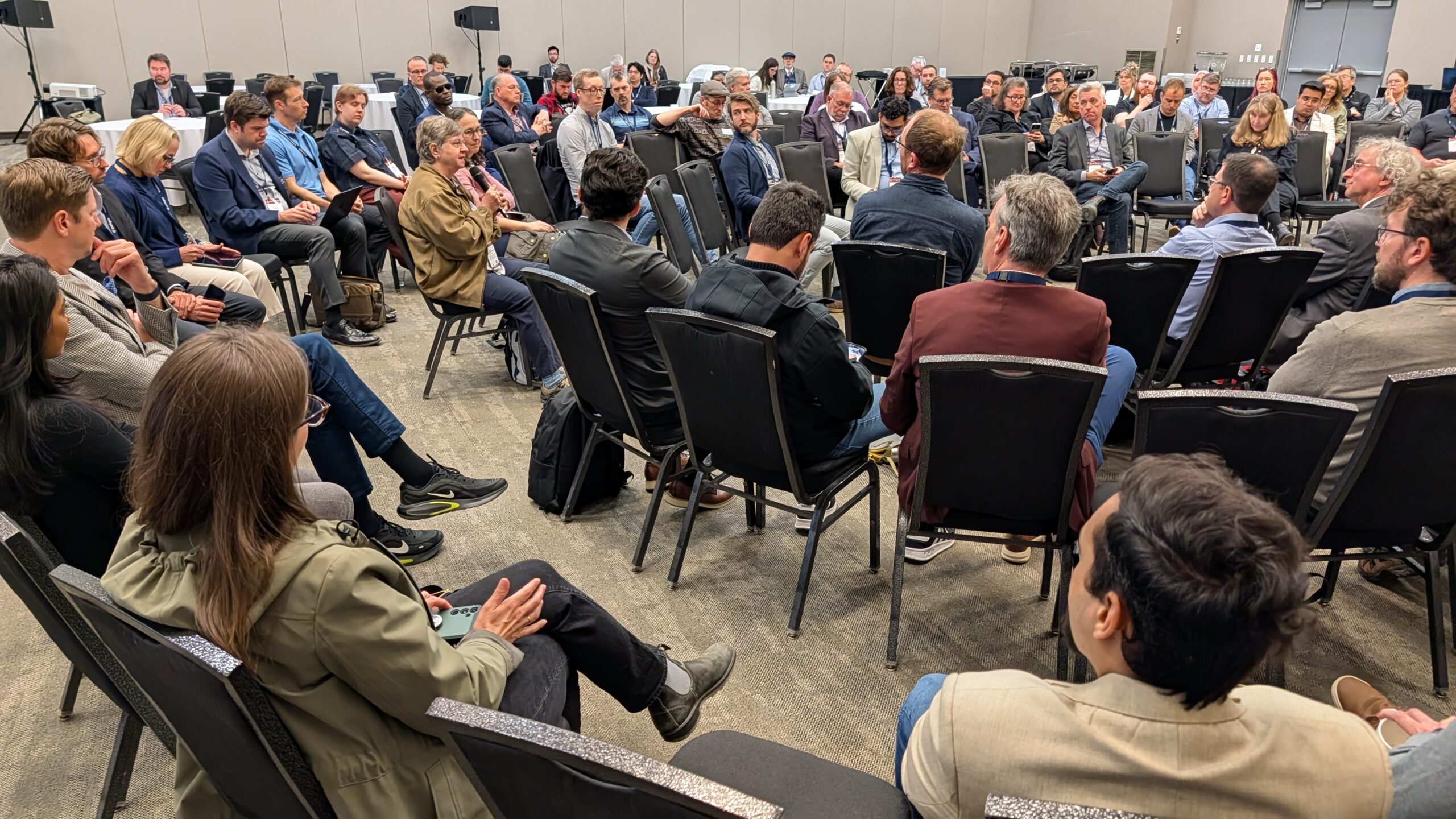

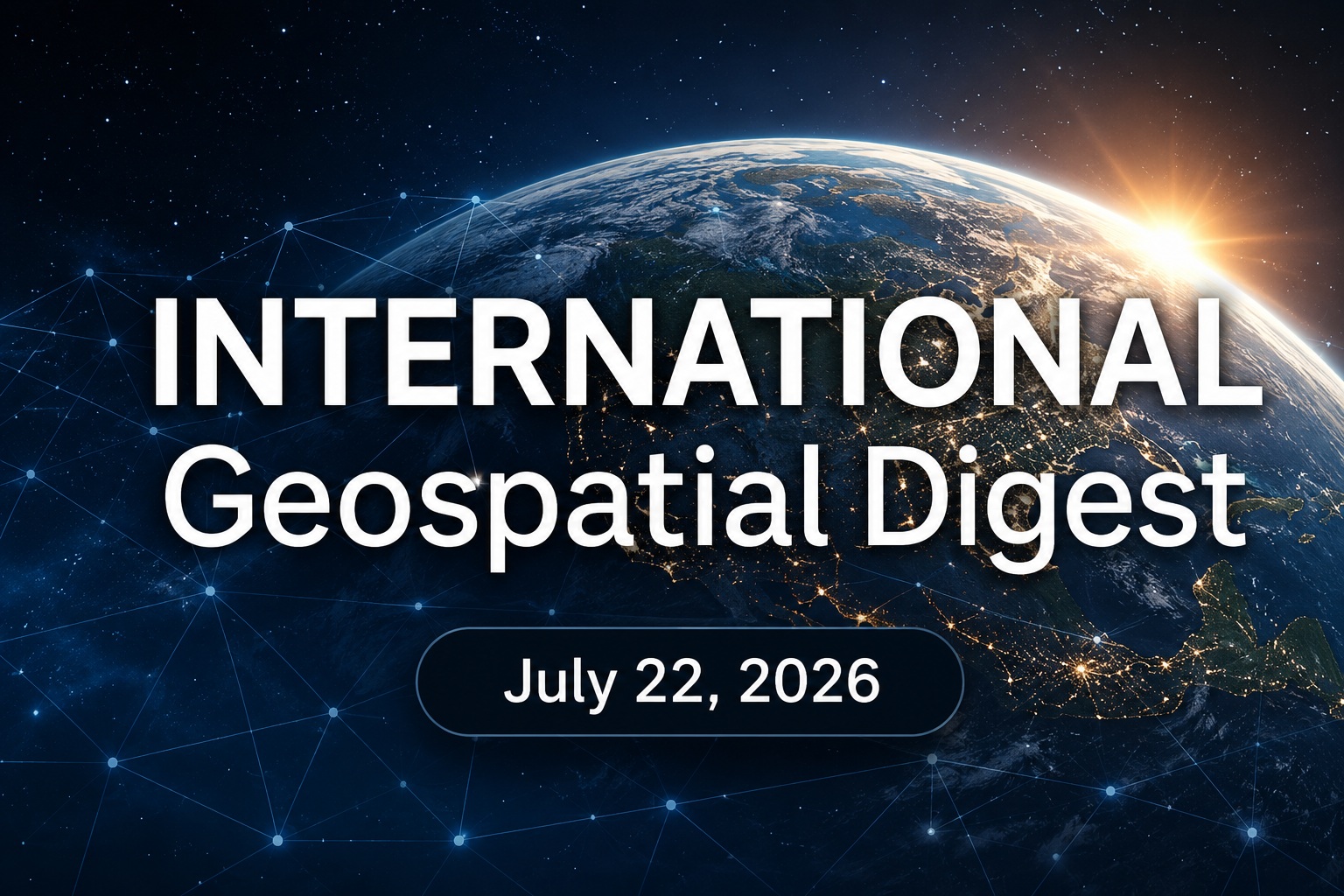
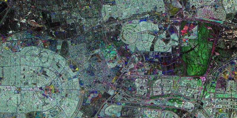


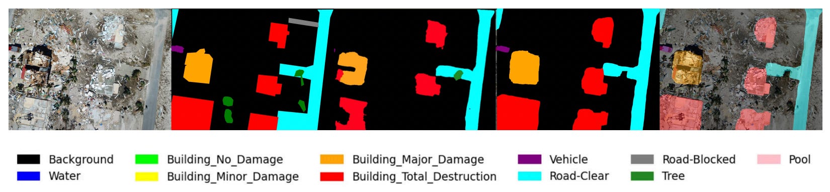


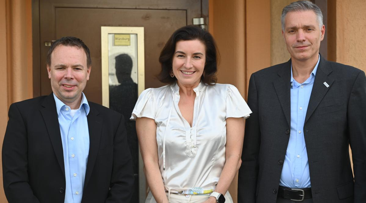


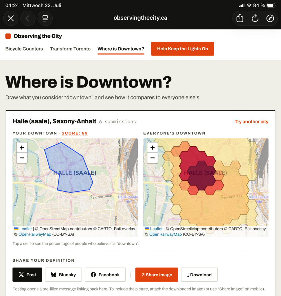


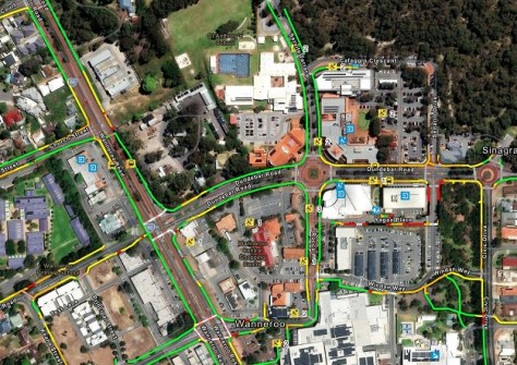

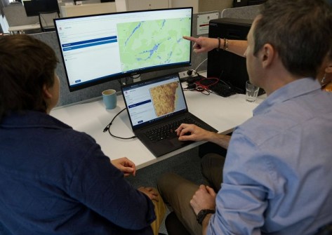

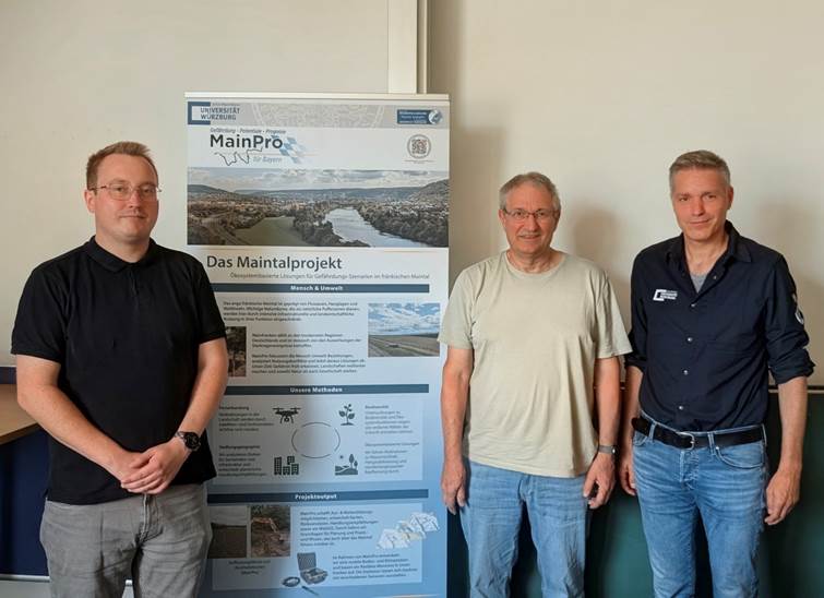

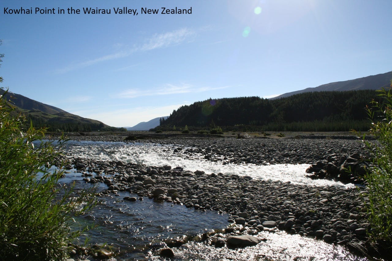
![EarthStuff - New Digital Tool Helps Farmers Boost Biodiversity In Scotland [spatial]](https://substackcdn.com/image/fetch/%24s_!OL1T!%2Cf_auto%2Cq_auto%3Agood%2Cfl_progressive%3Asteep/https%3A%2F%2Fsubstack-post-media.s3.amazonaws.com%2Fpublic%2Fimages%2Ff1003ffd-80f5-43eb-9978-0ec377fb691e_3200x1800.jpeg)
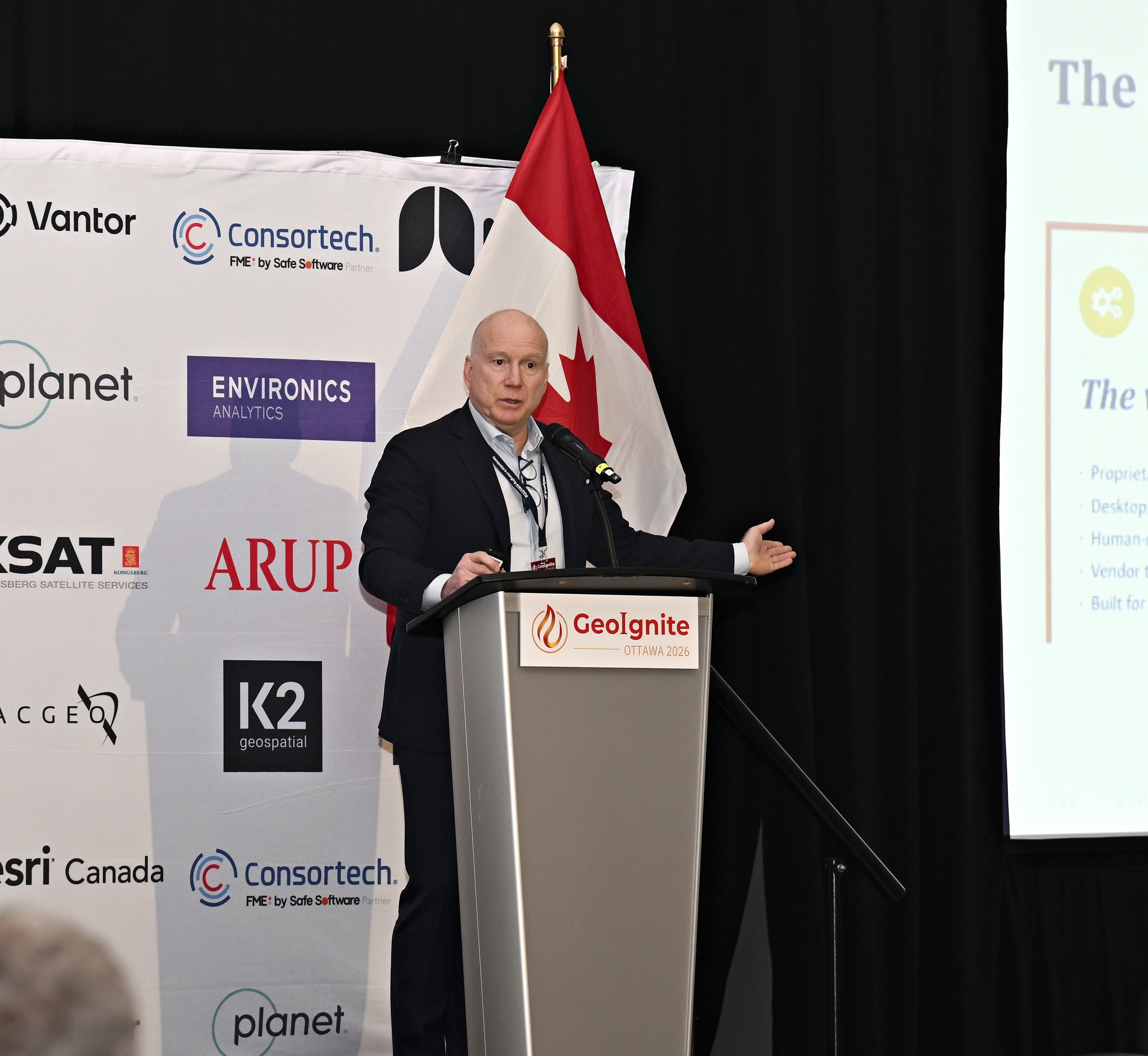


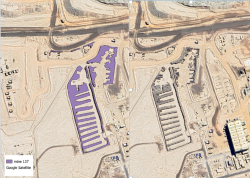

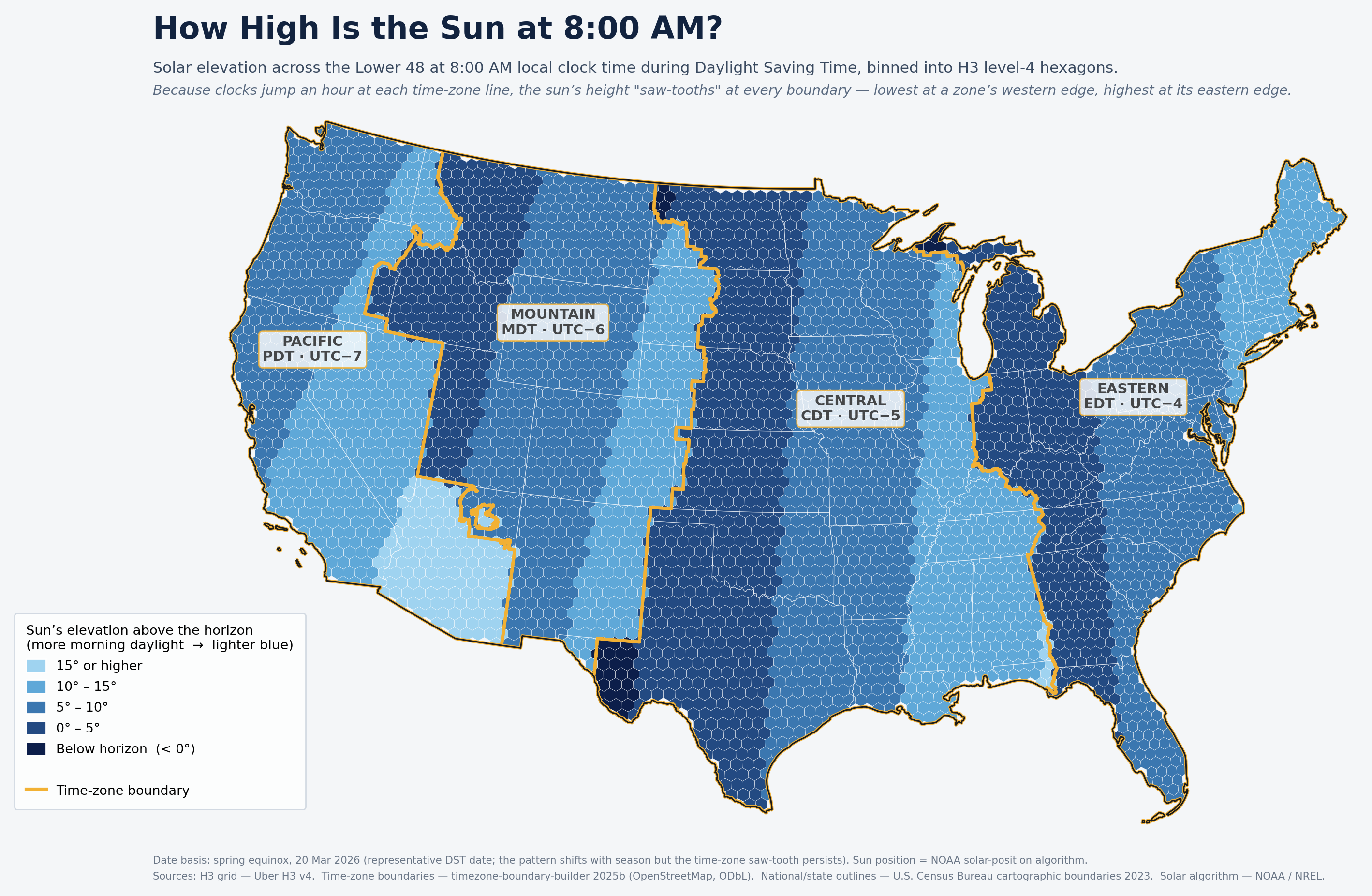

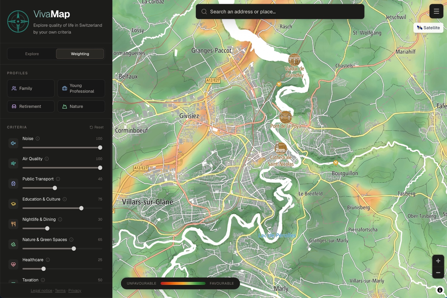


.gif)


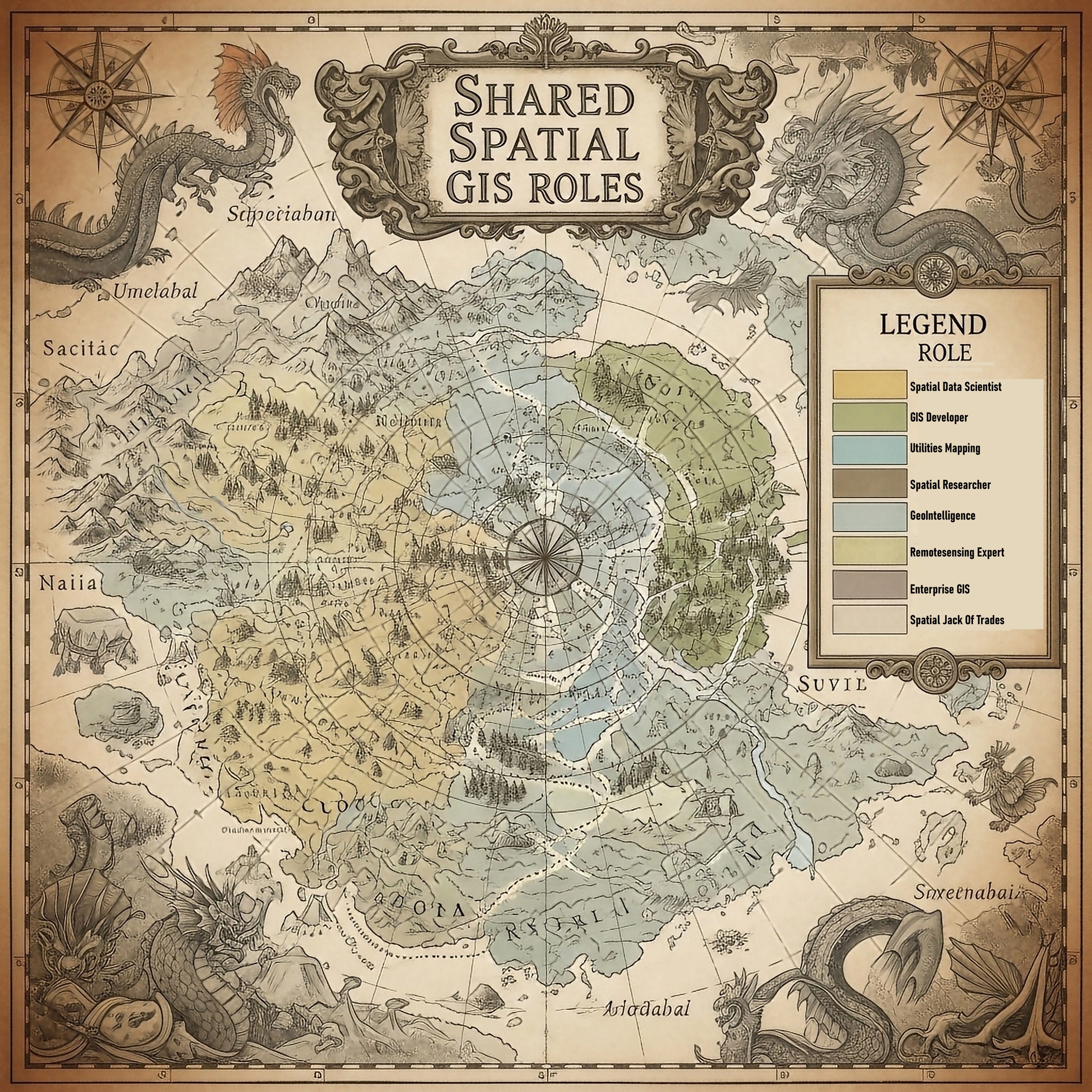


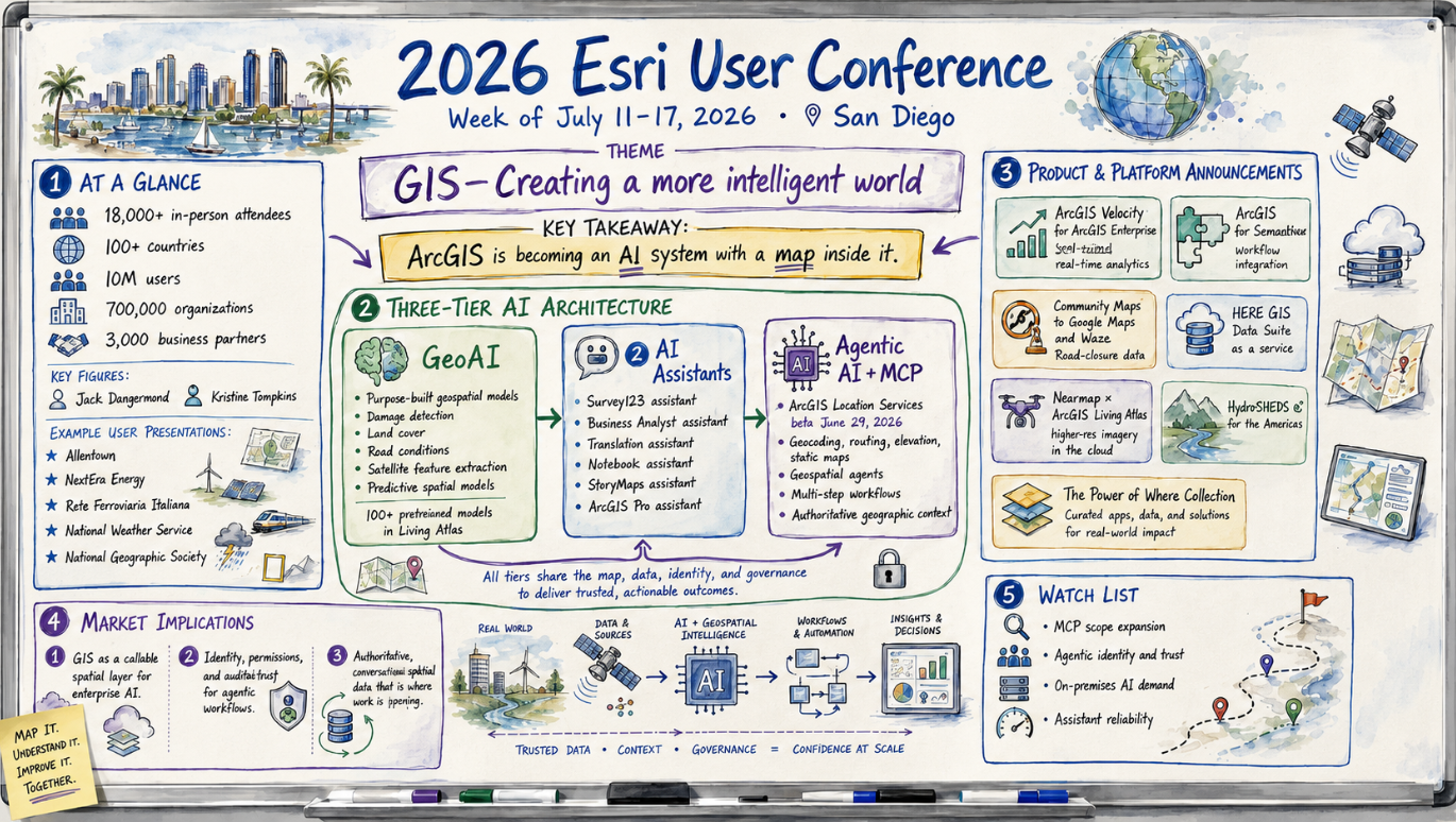
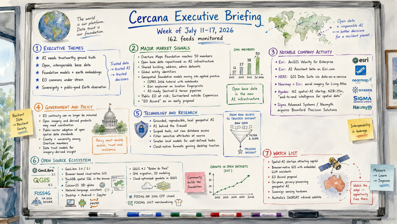
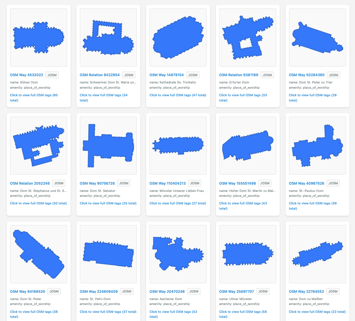
.gif)

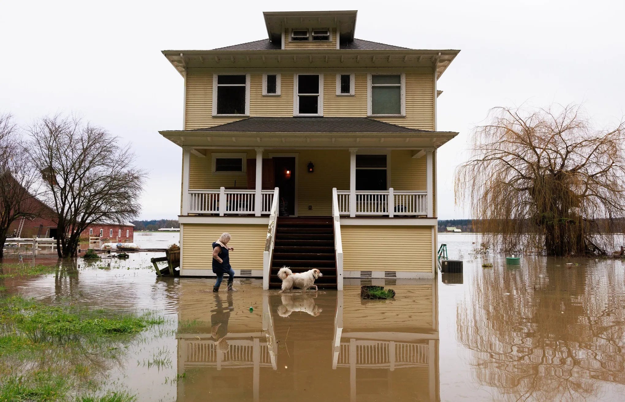
![Mergin Maps case studies - [QGIS] Mapping 8,000 km of Tuscan waterways: How GAIA digitised its water network](https://cdn.prod.website-files.com/64be358a4fb0e612b228bb9e/6a5f7d0231f705736935bcf6_survey_02_cut.jpg)
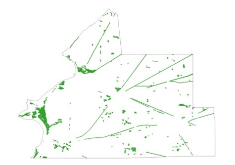

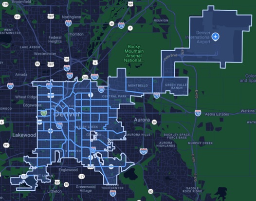

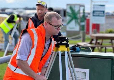
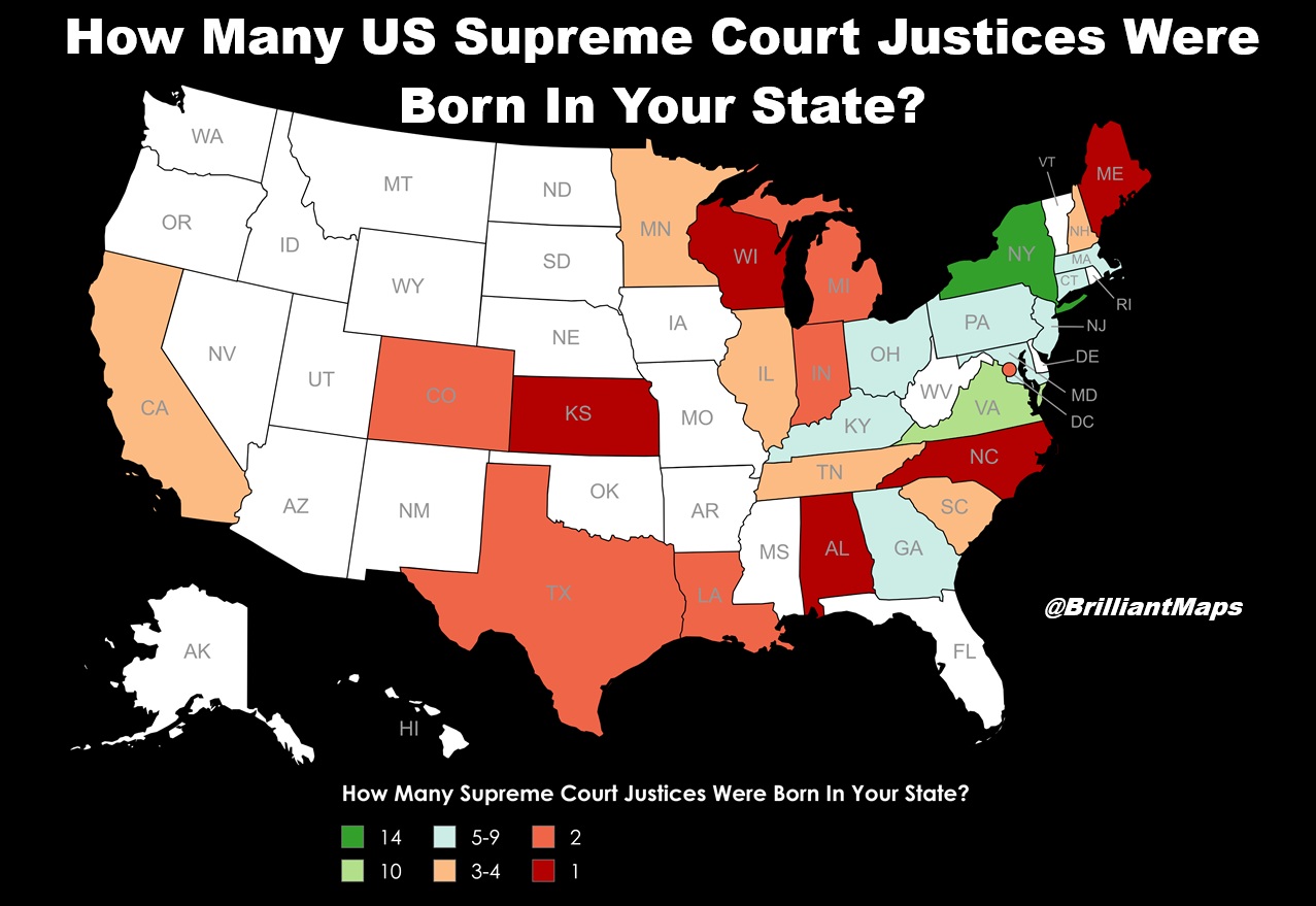


.jpg)
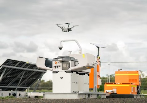


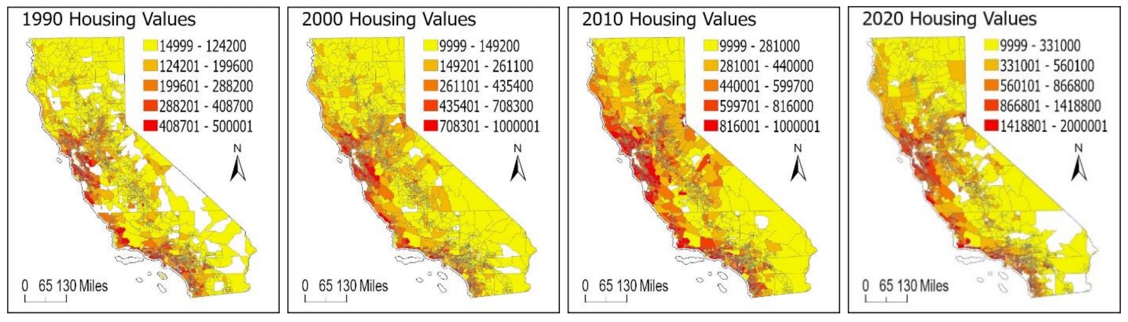
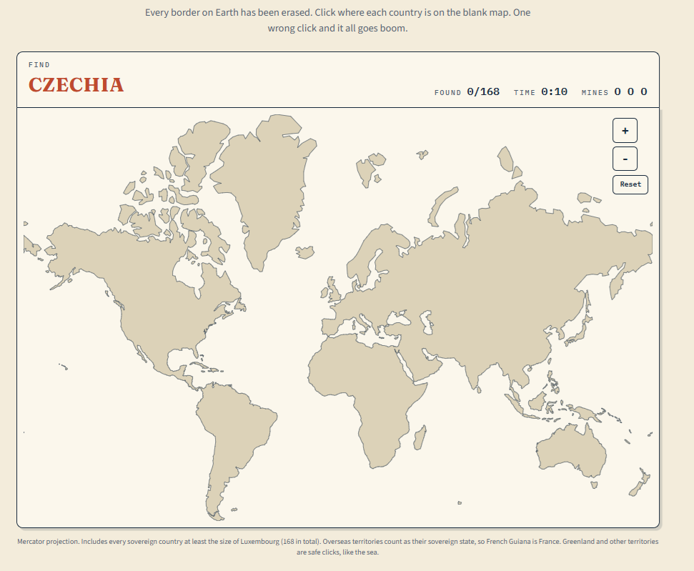

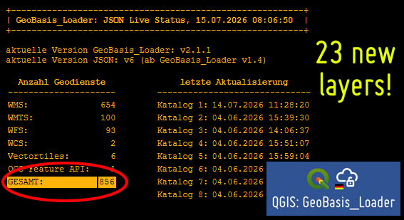
.gif)


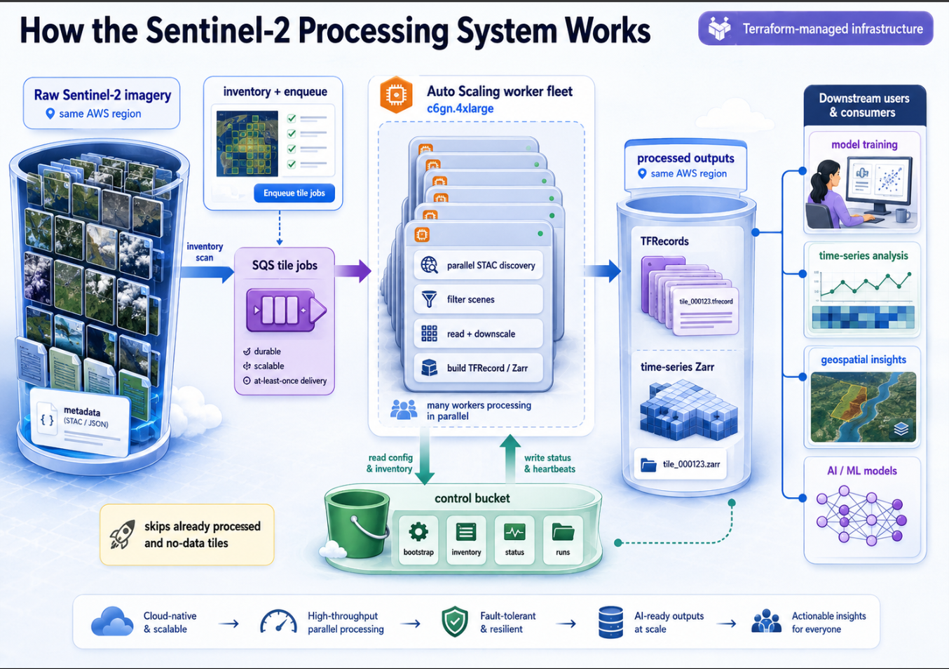
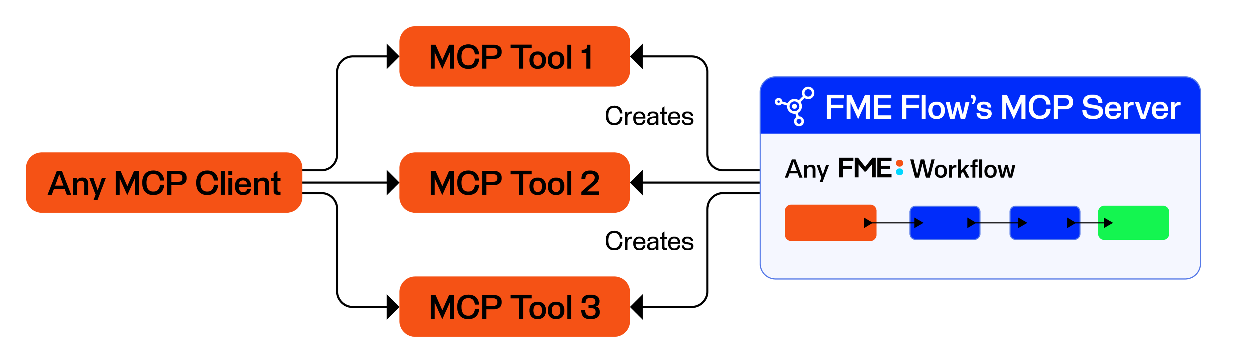

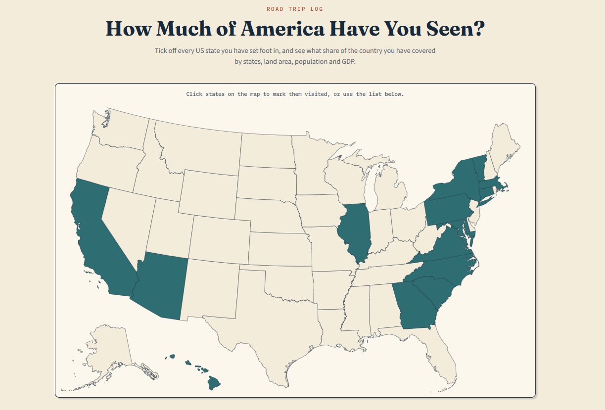
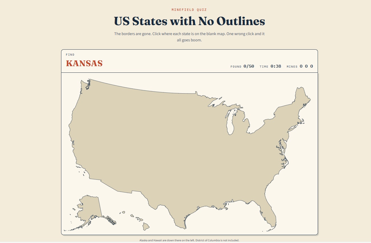
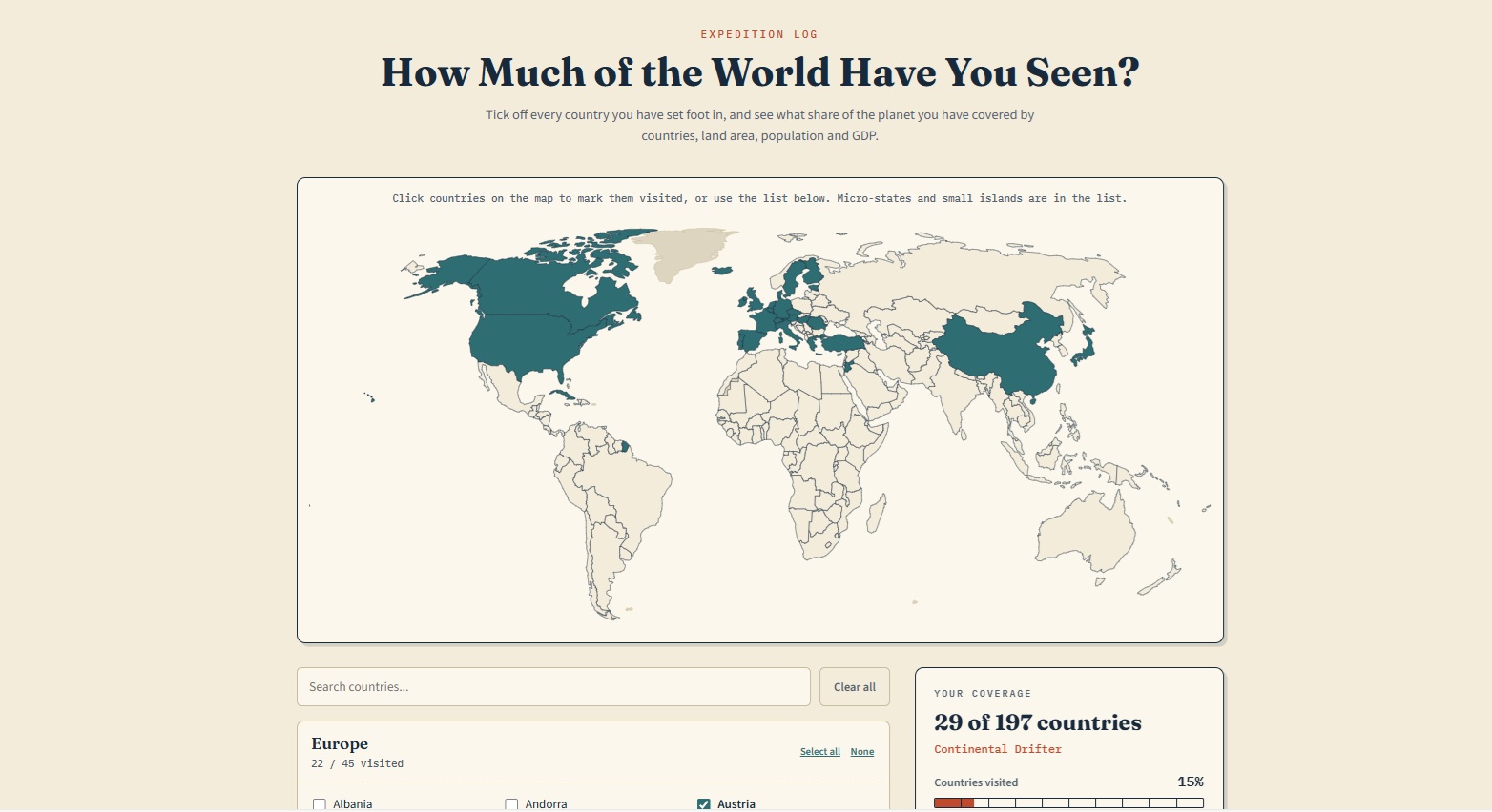

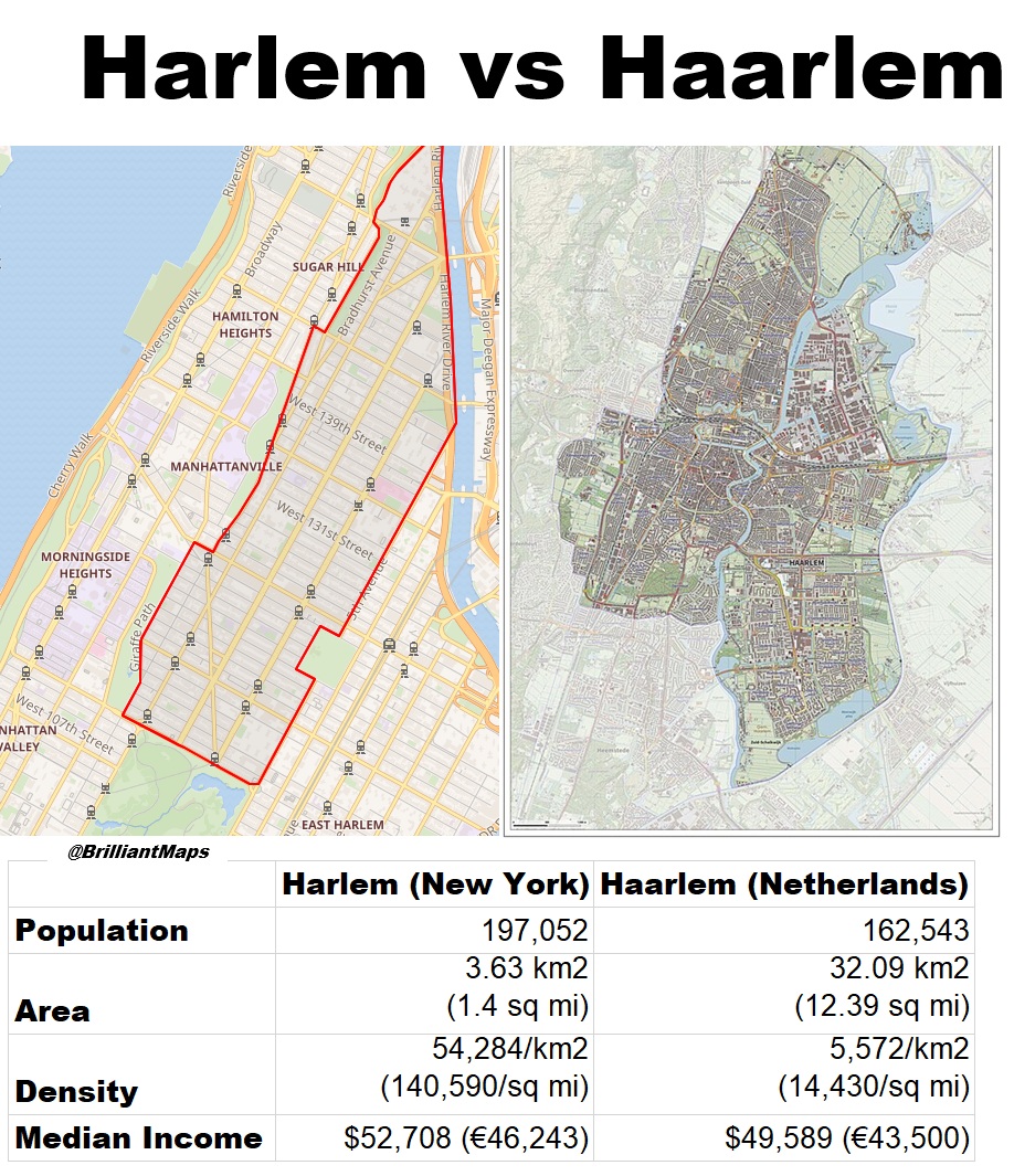


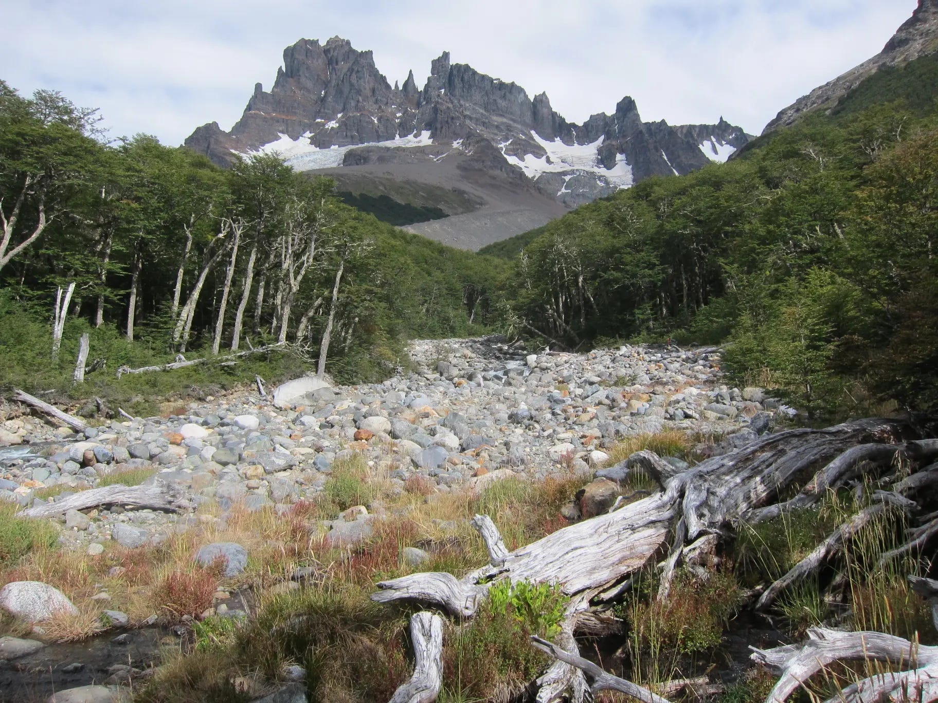


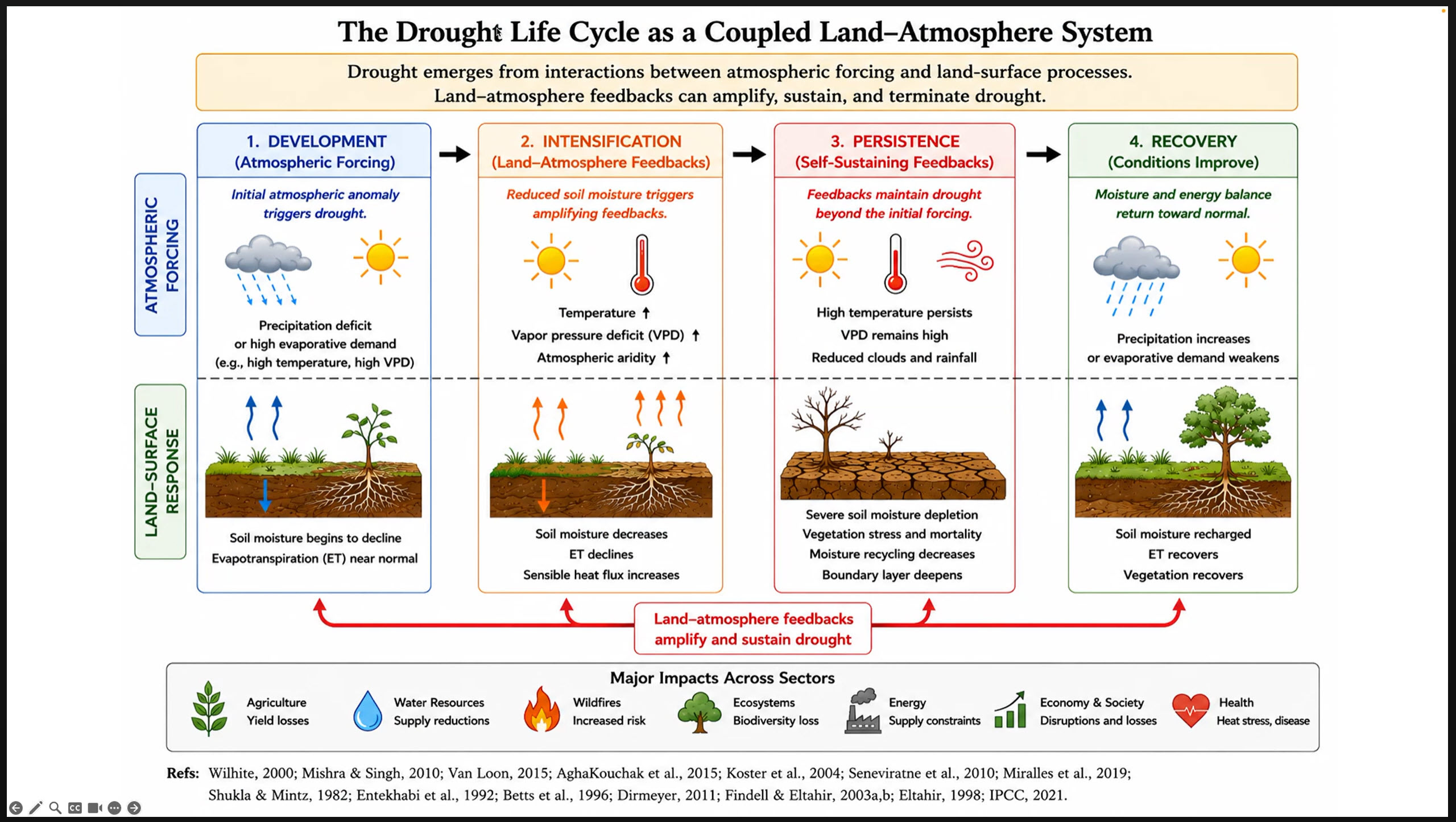
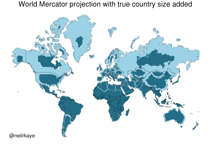


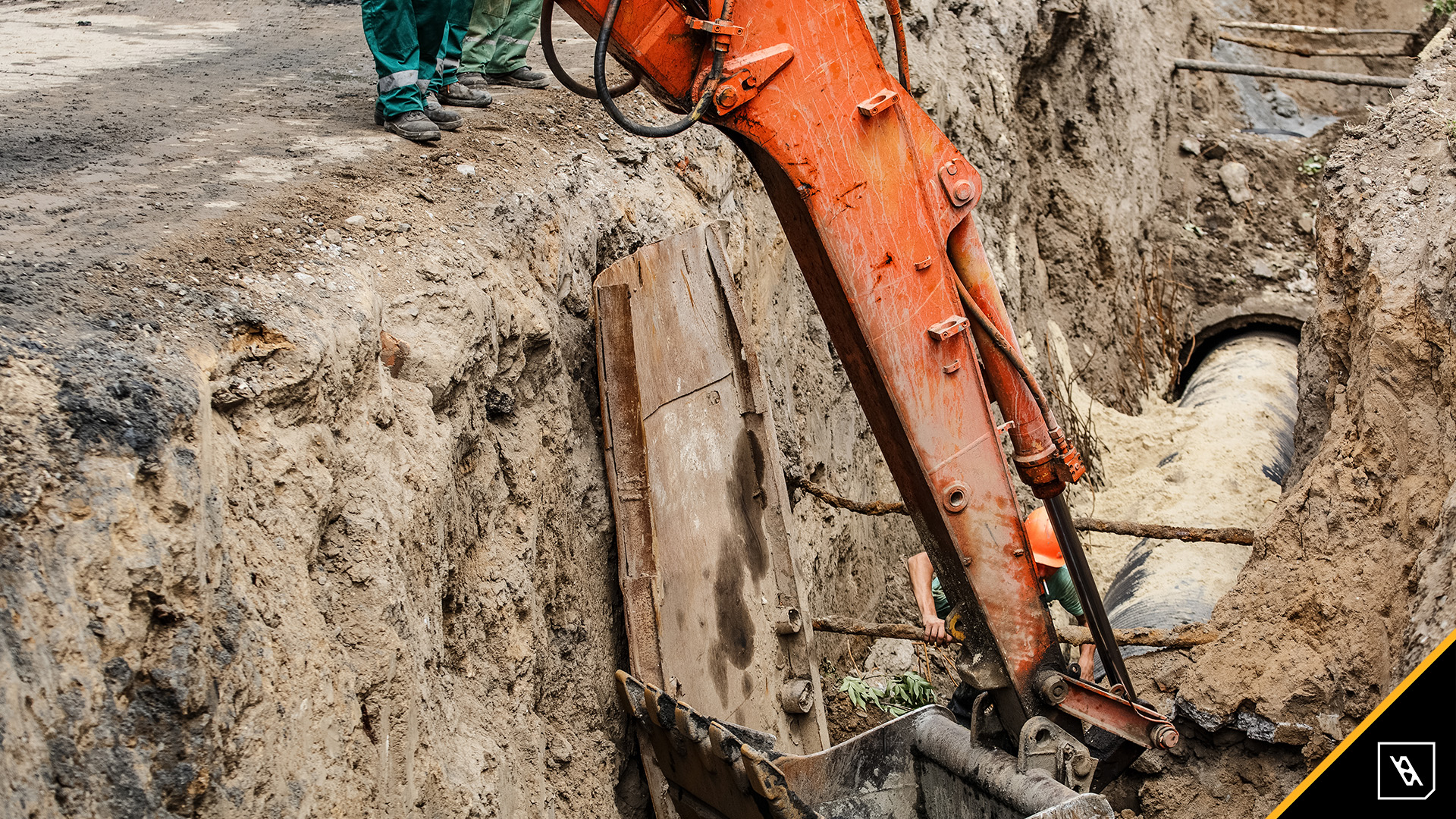


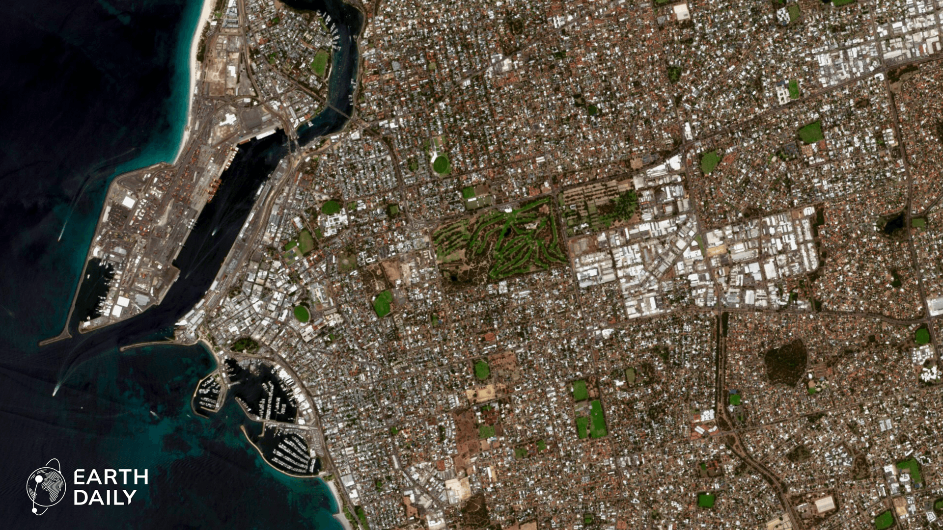


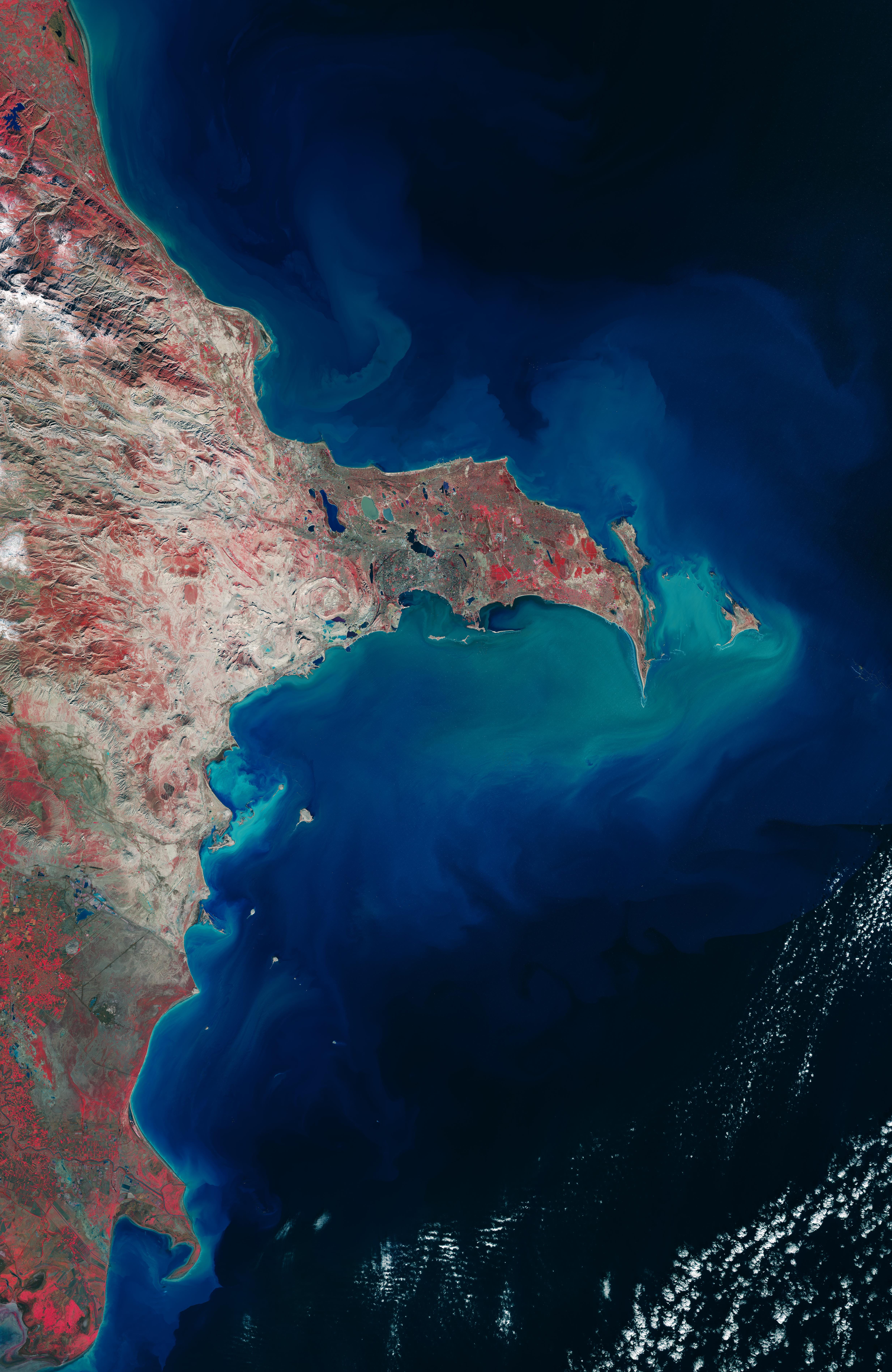

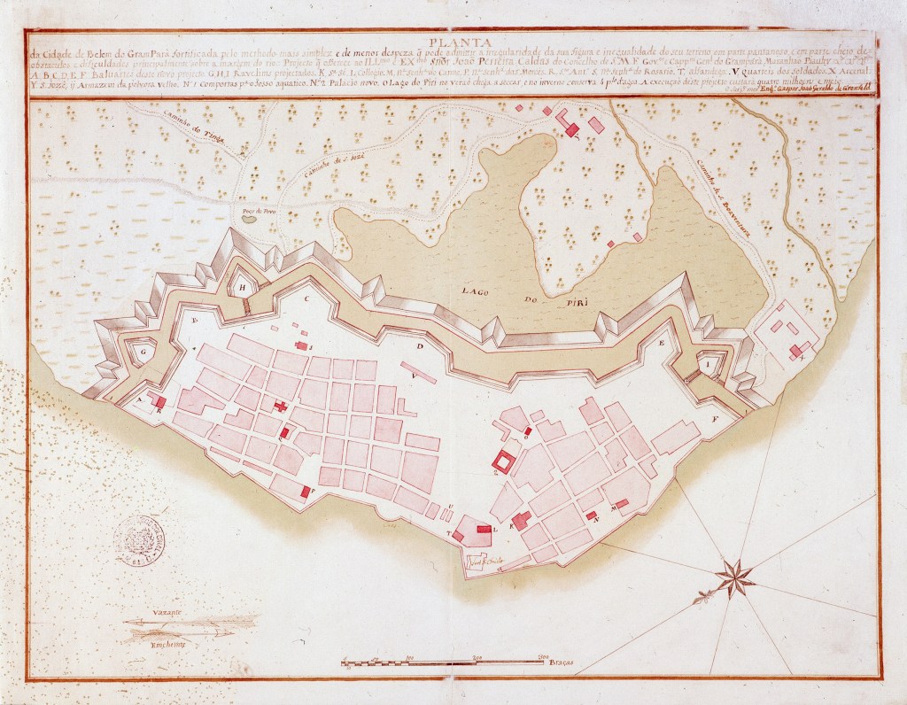


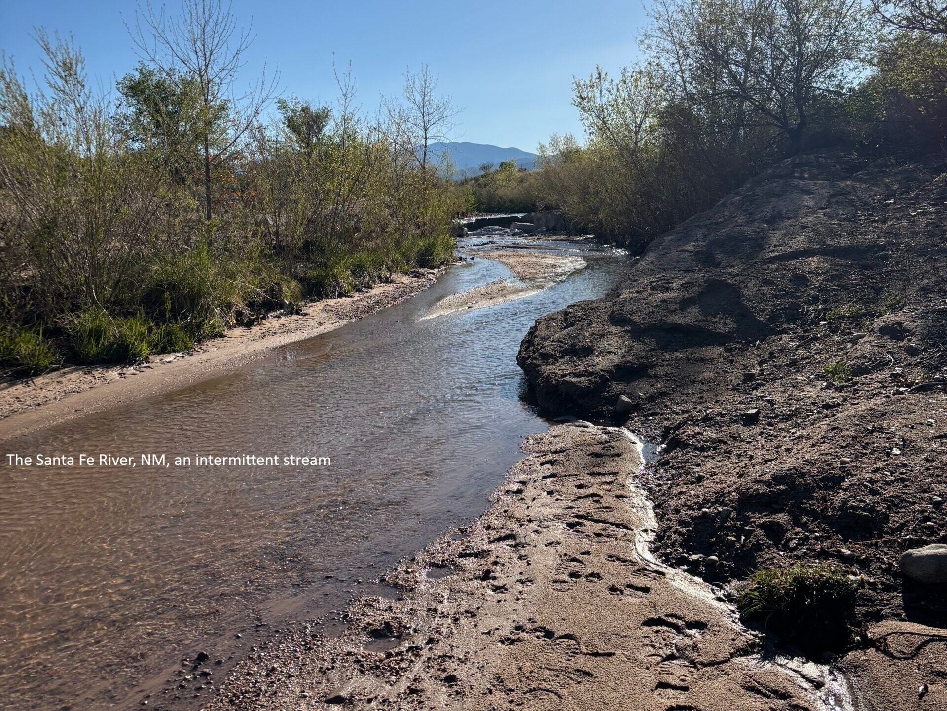

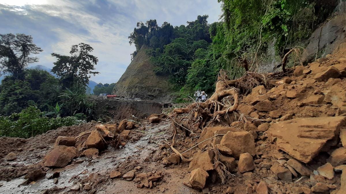
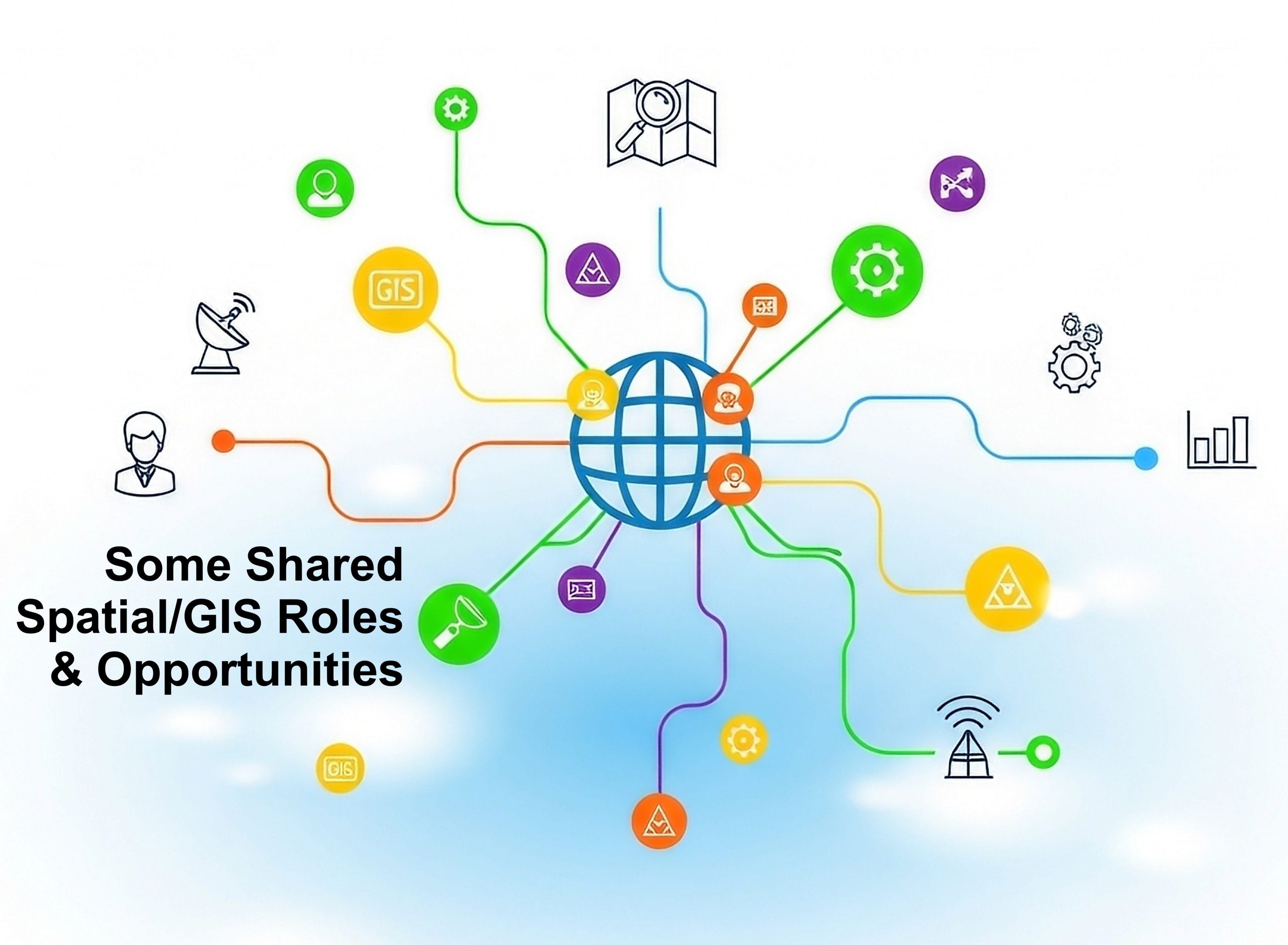


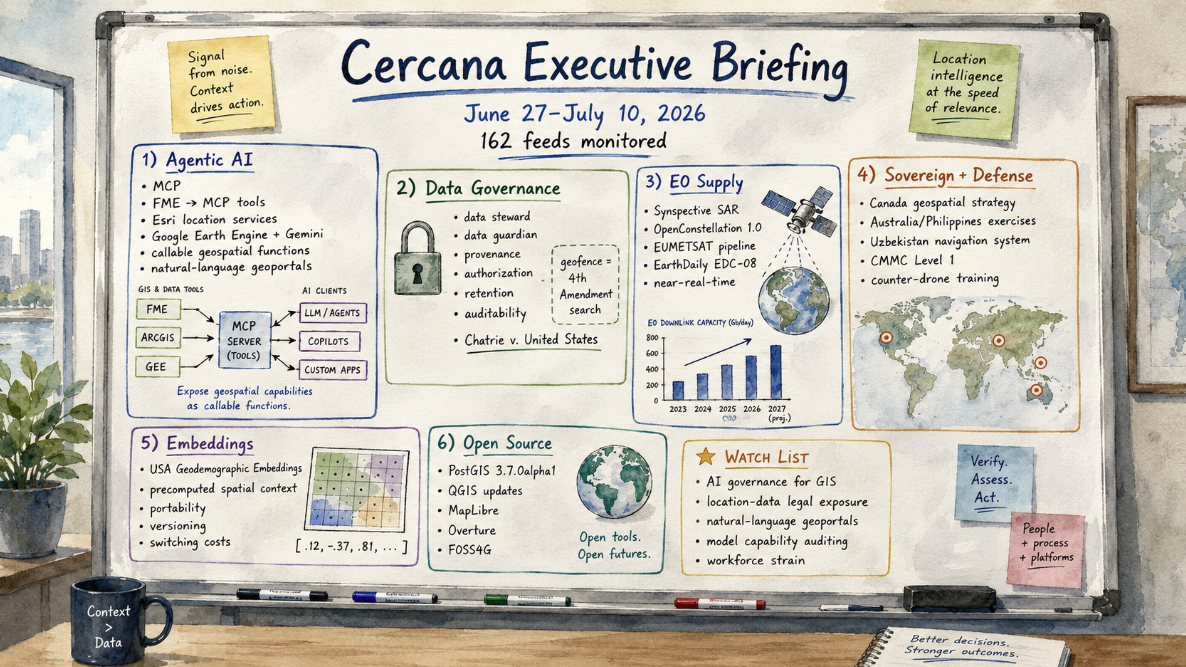


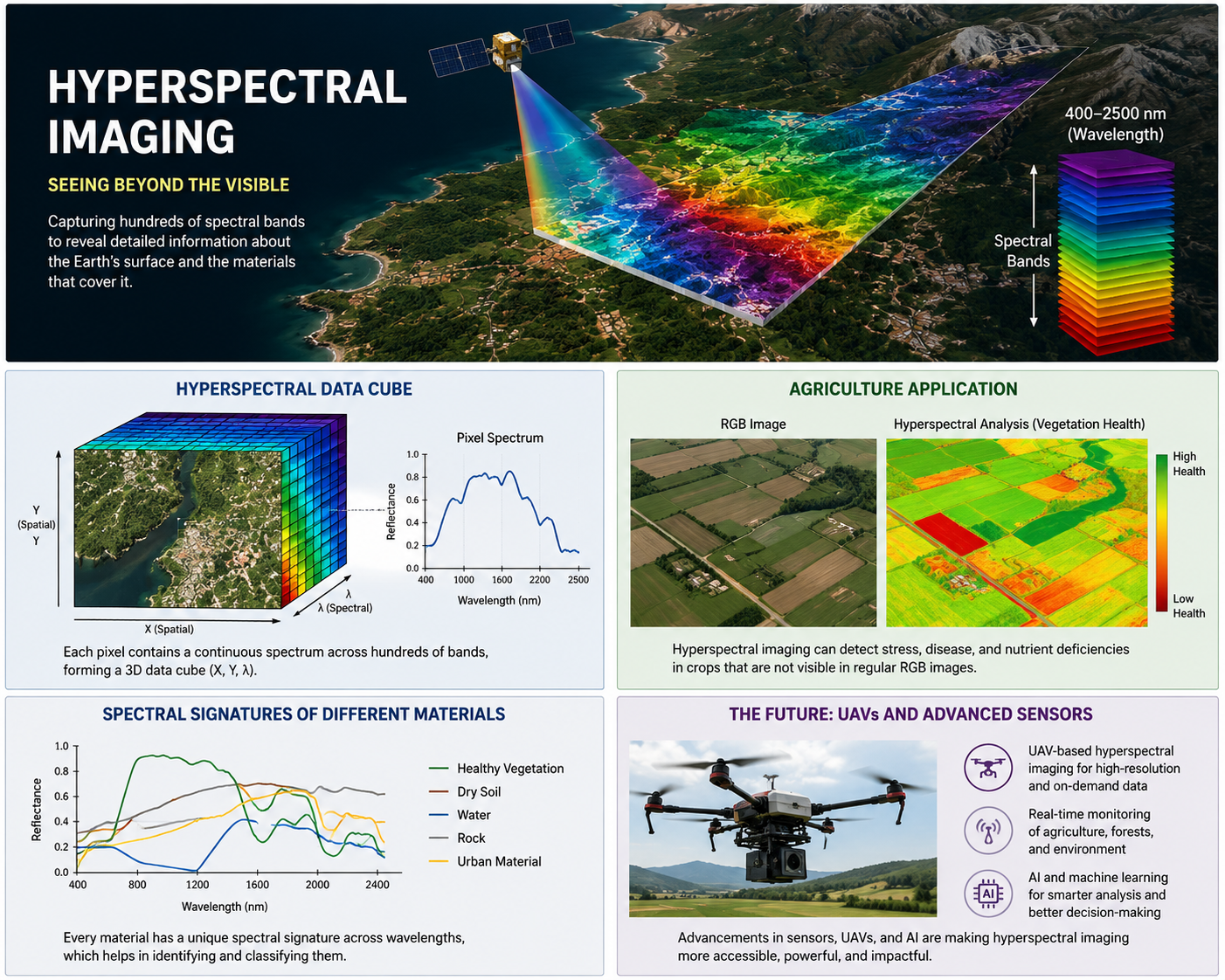


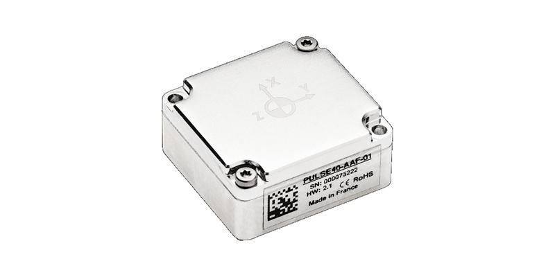


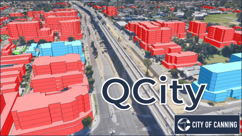
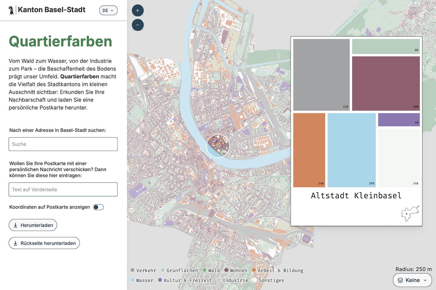

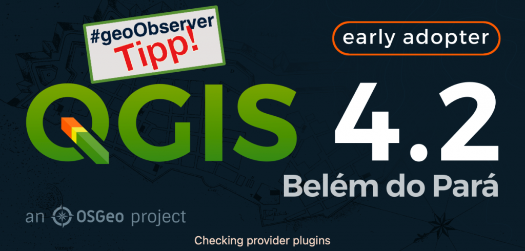

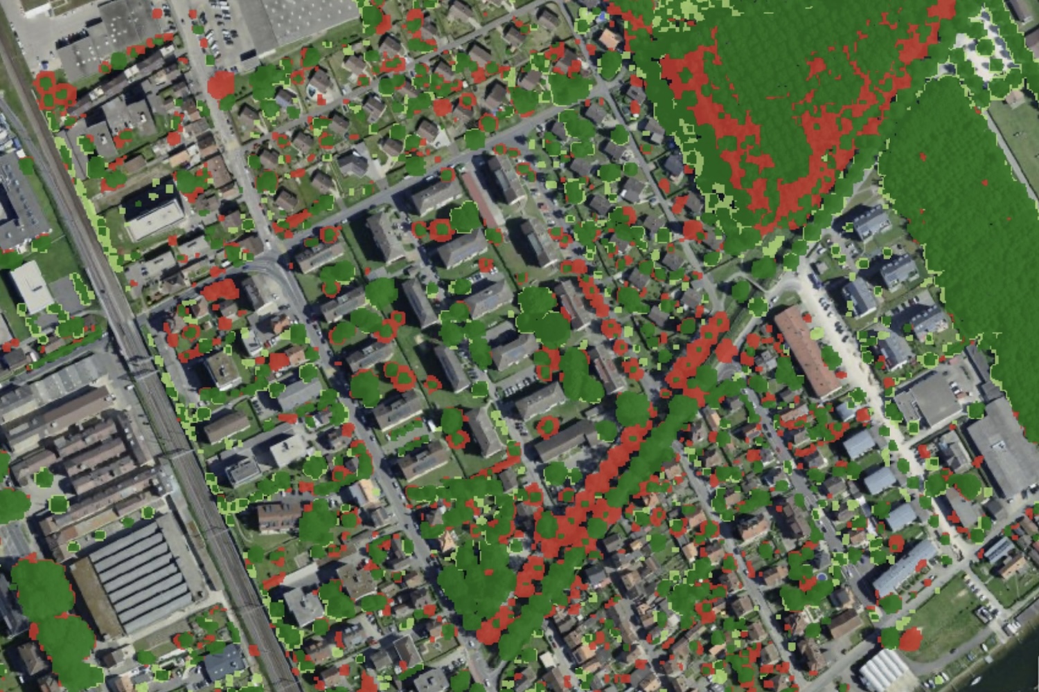
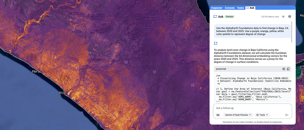


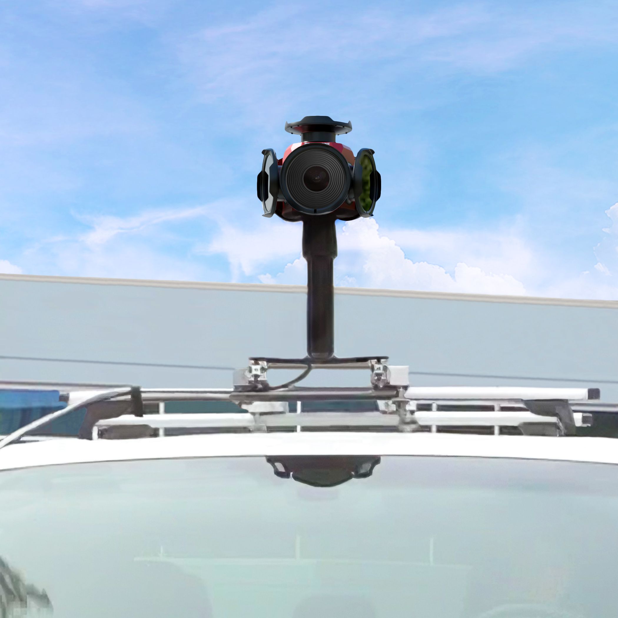

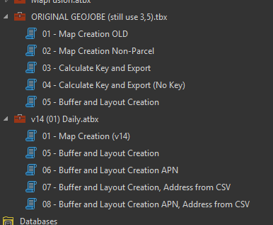

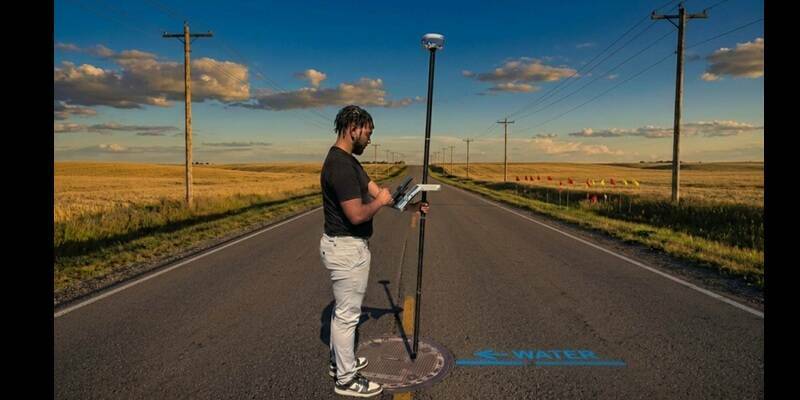


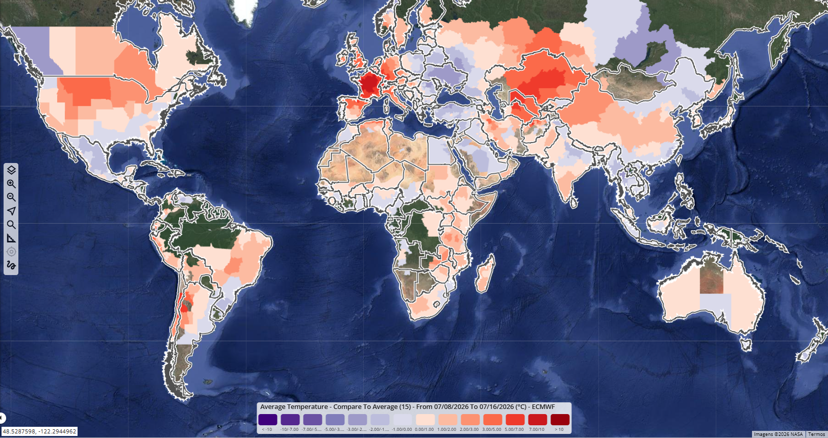


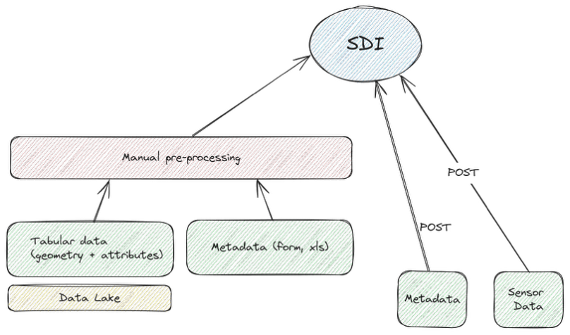


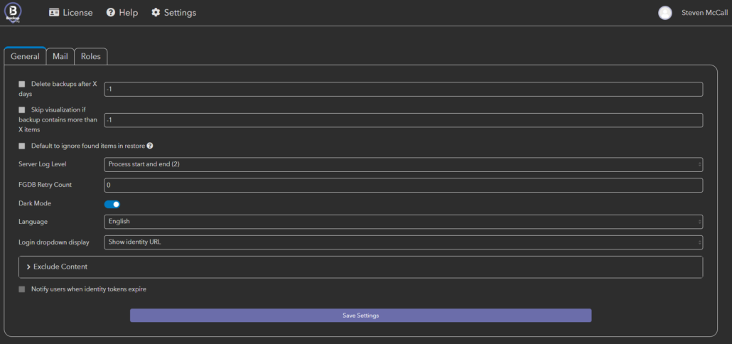
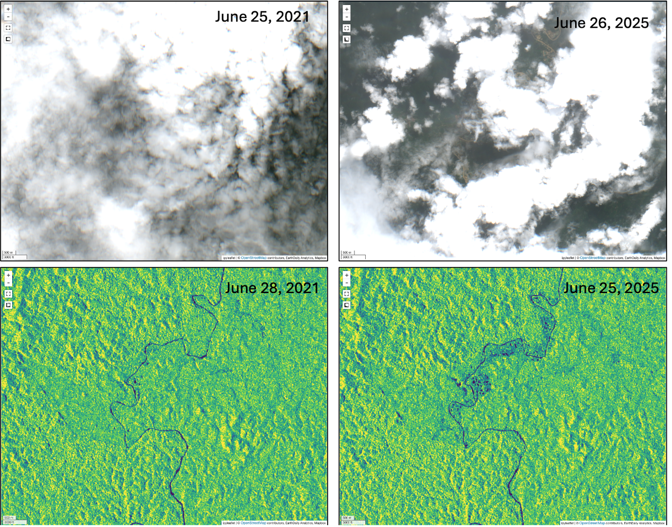
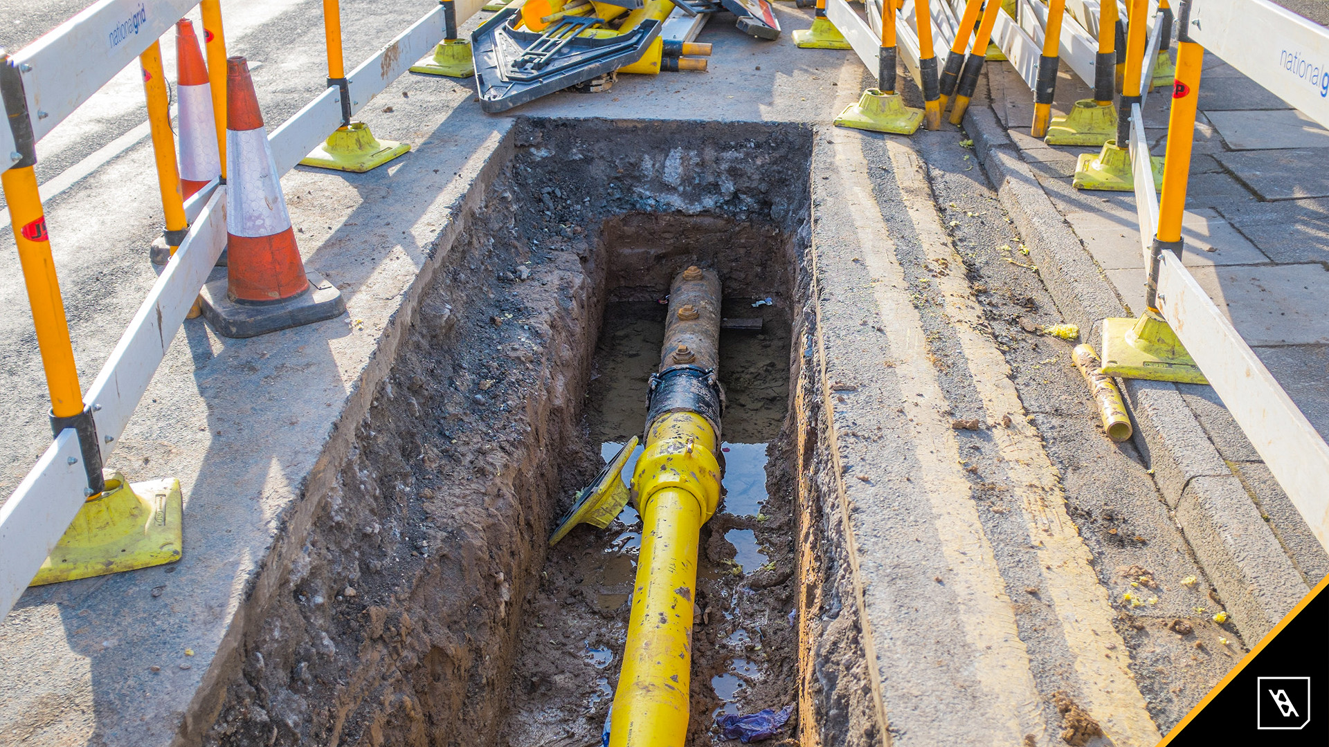


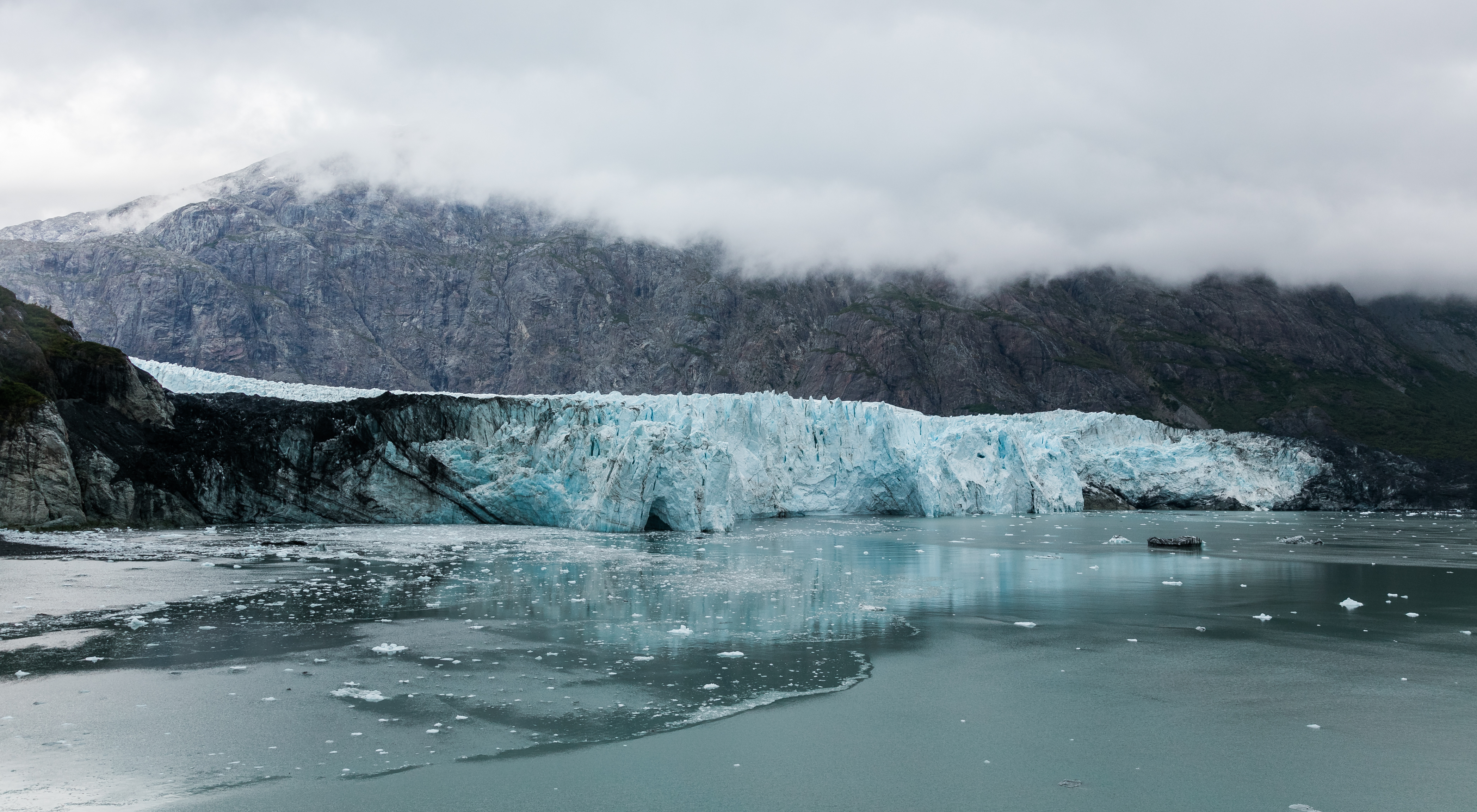


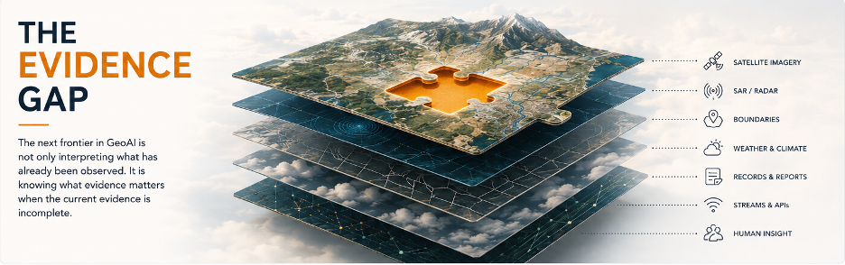


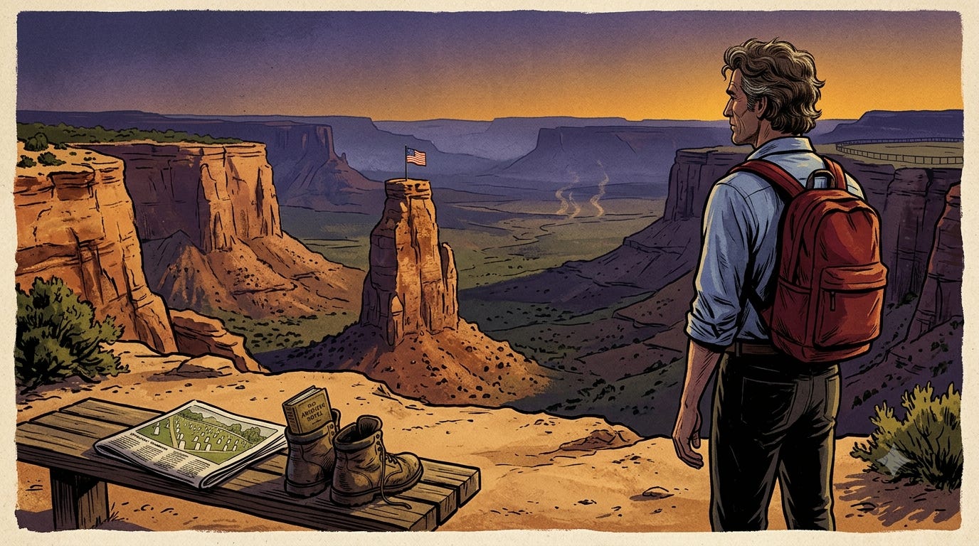
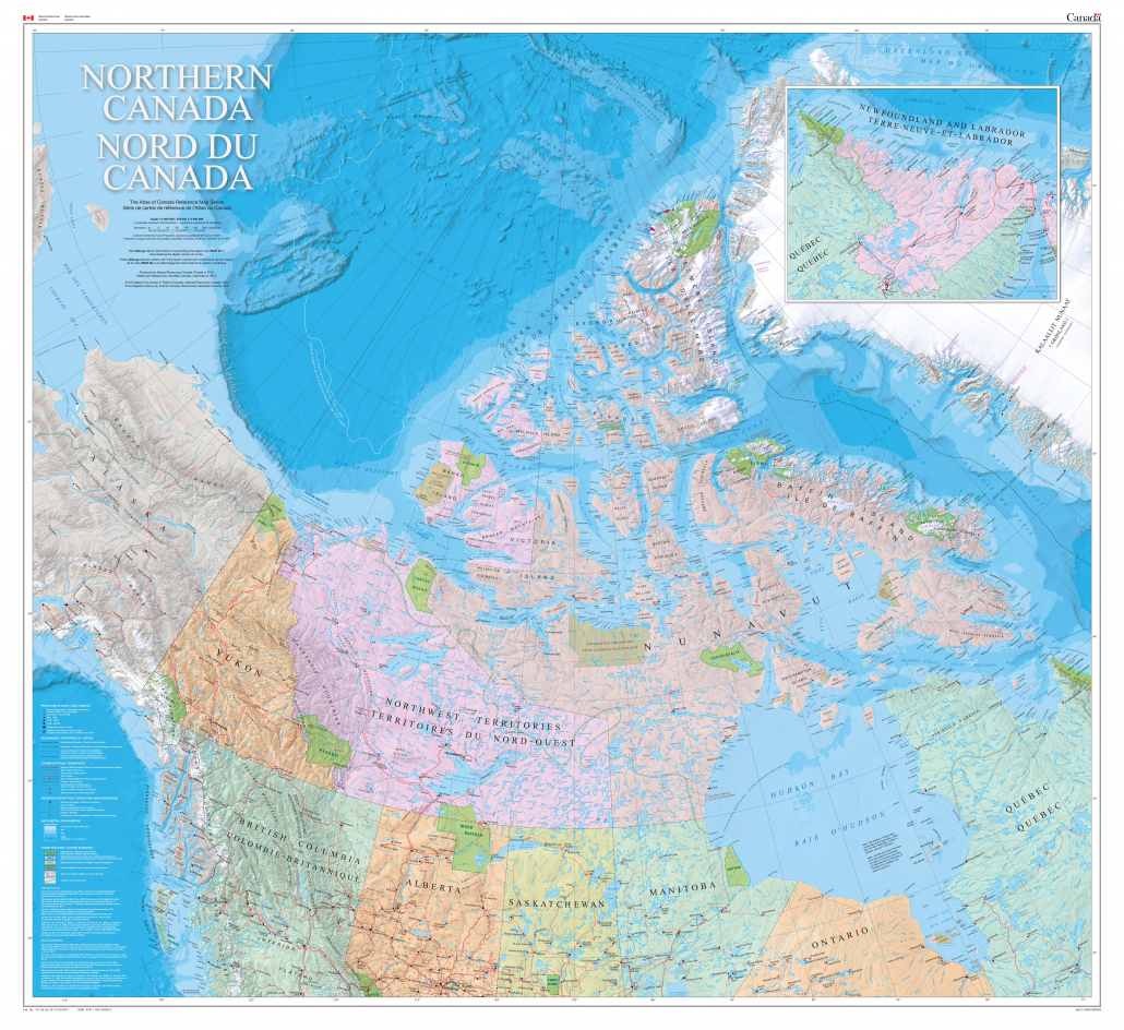


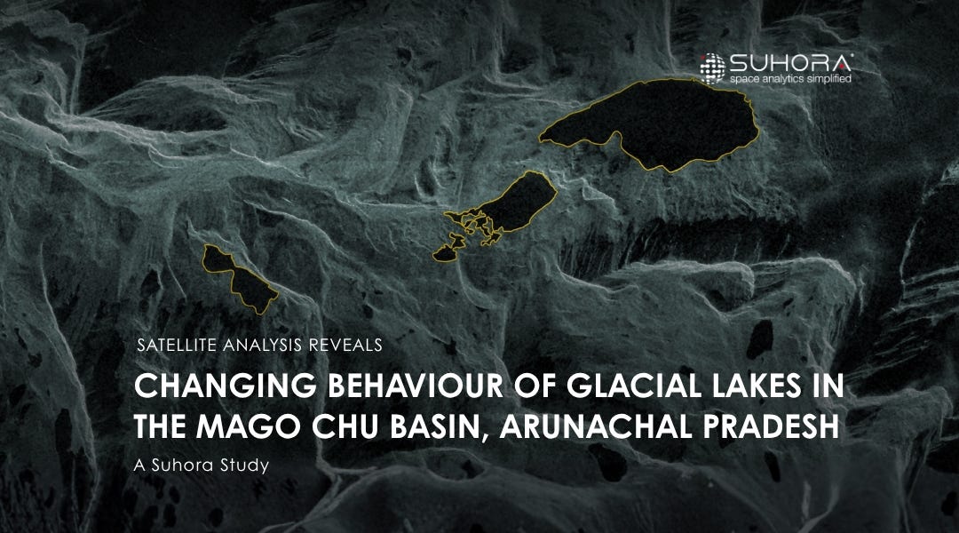


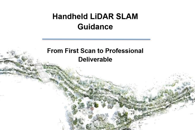


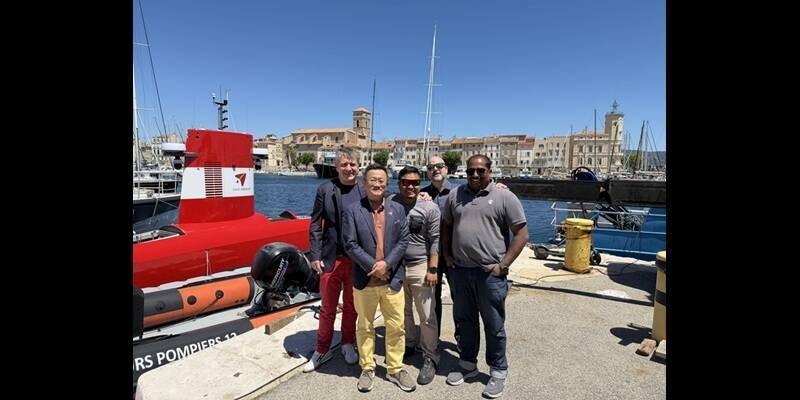
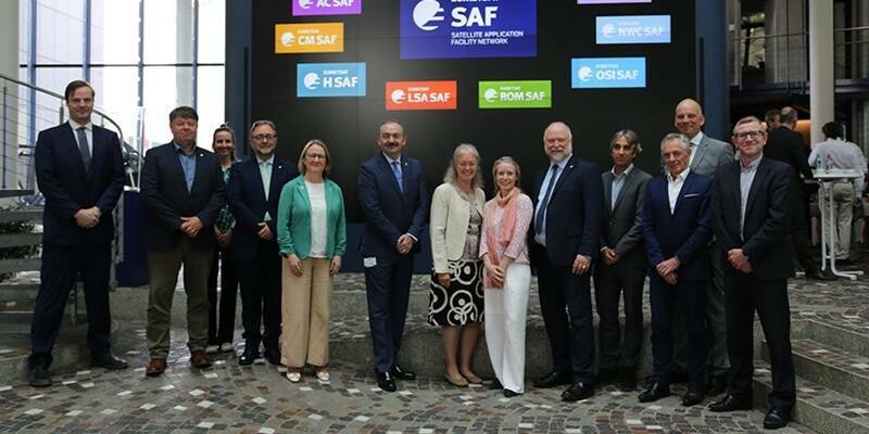

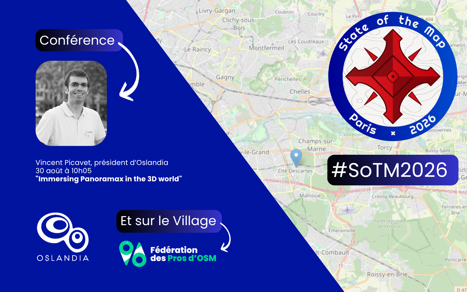


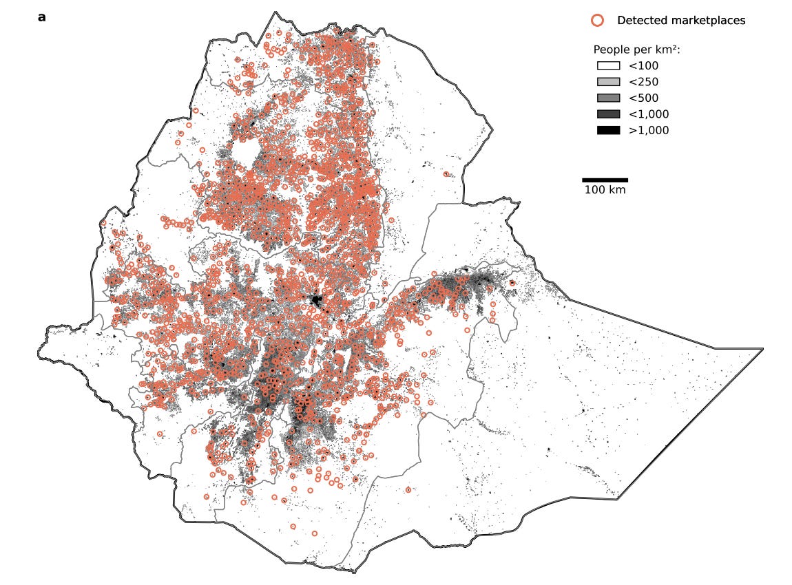


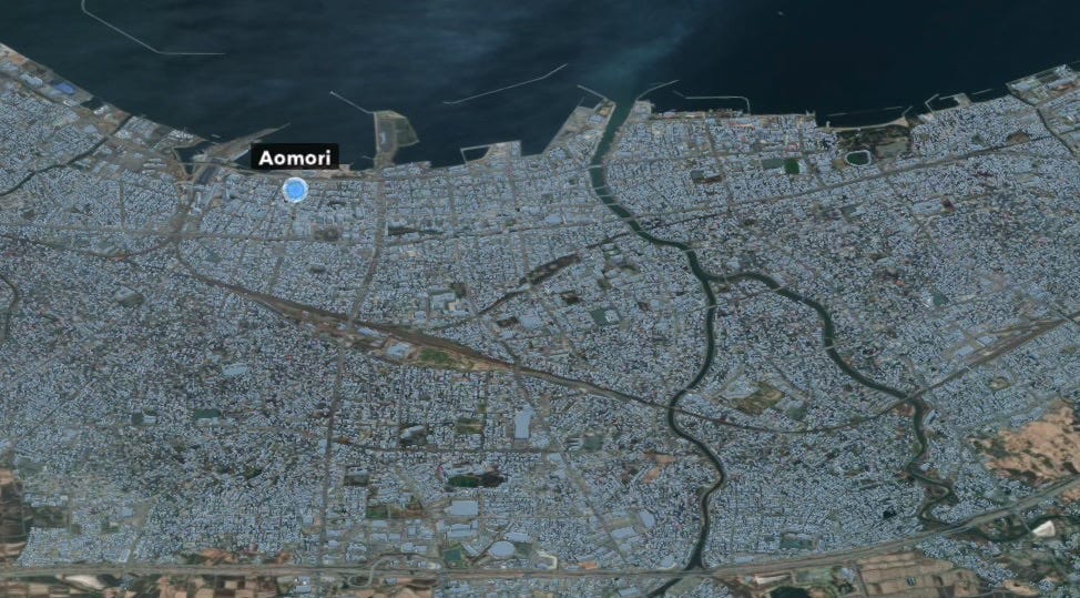


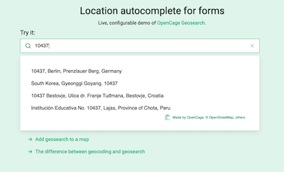


.png)
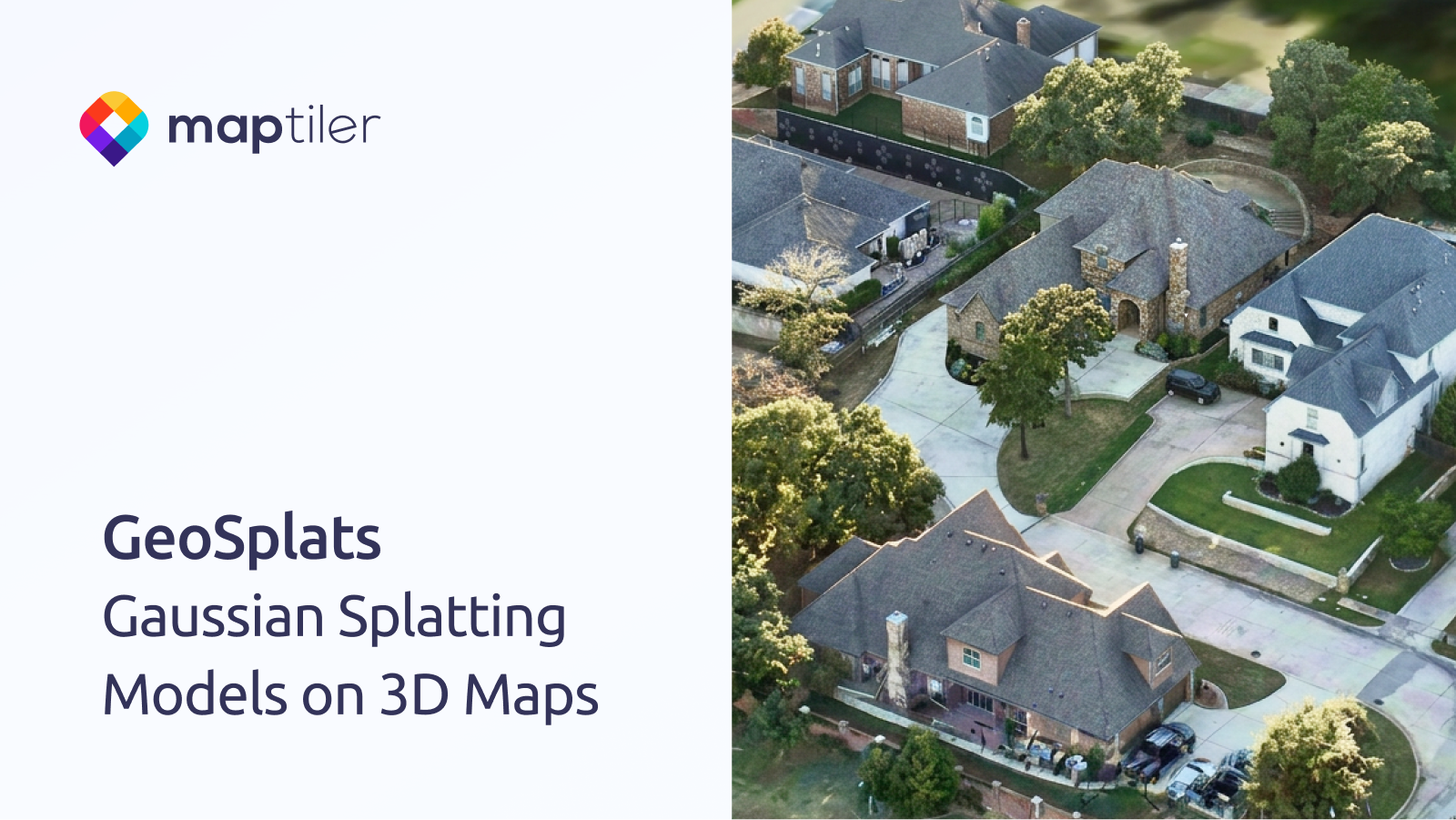


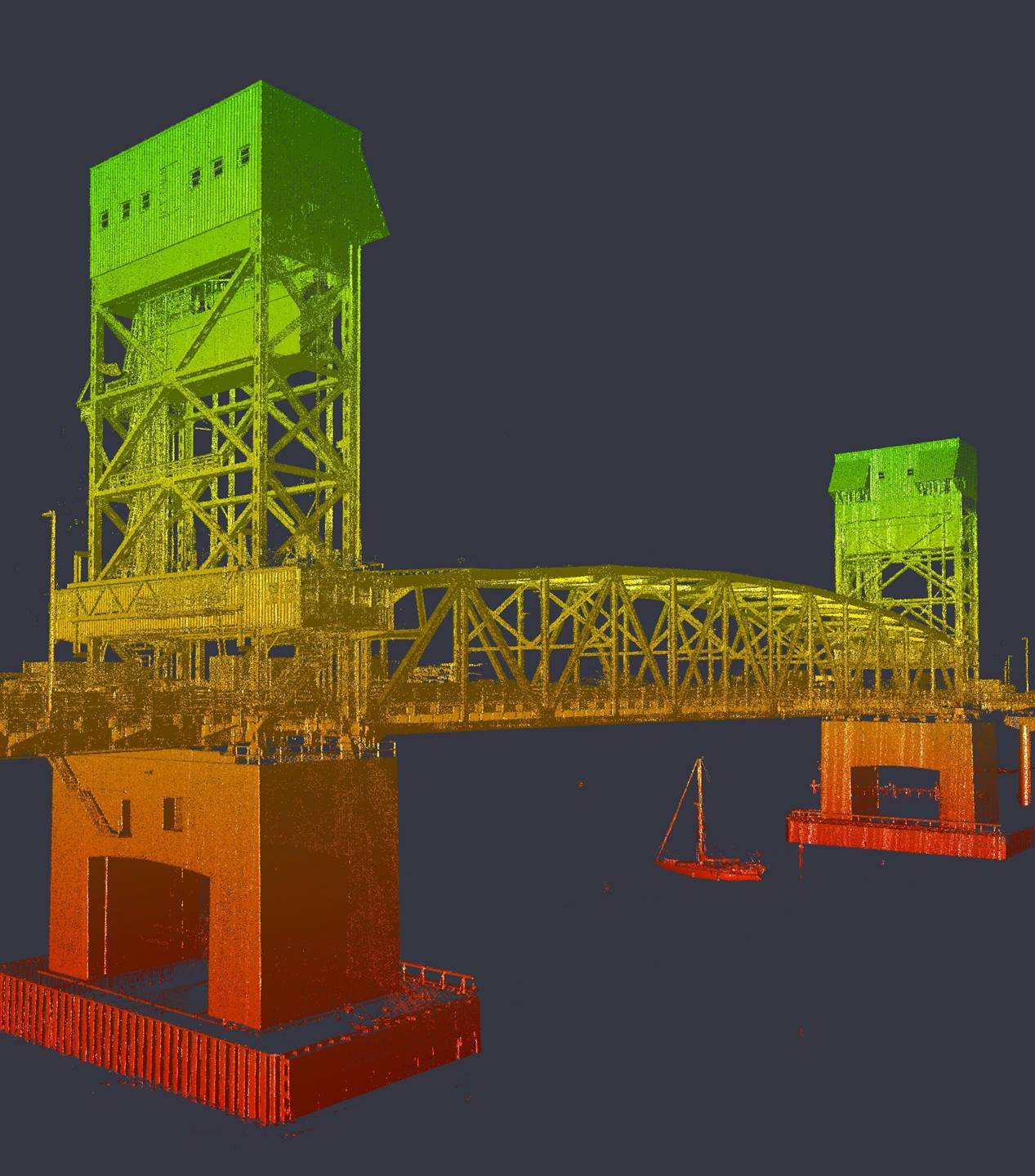

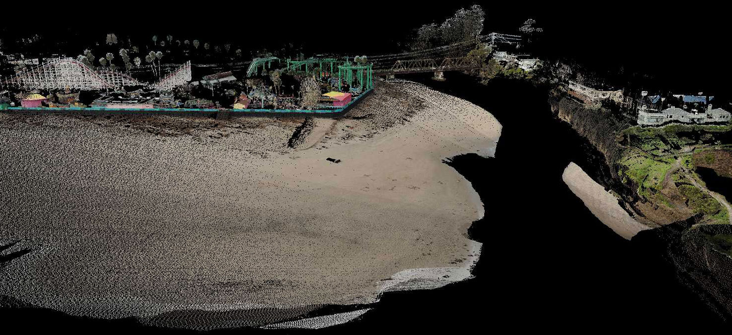
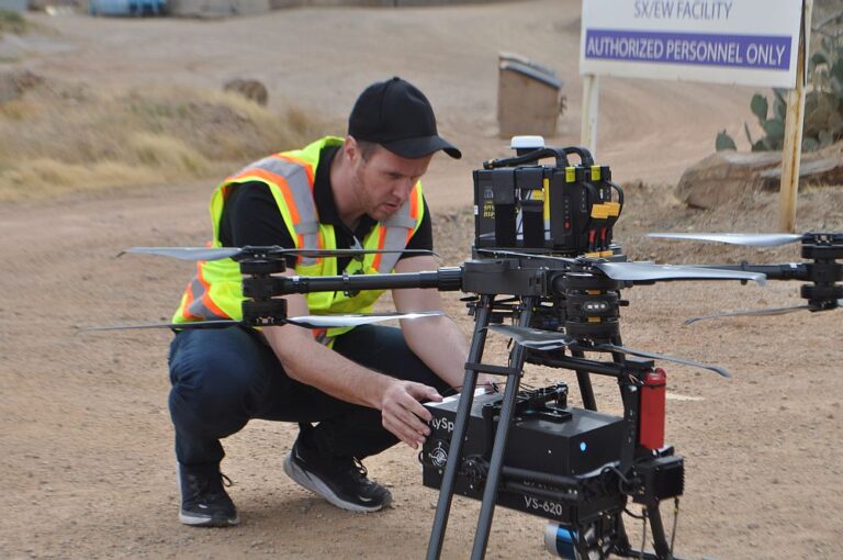


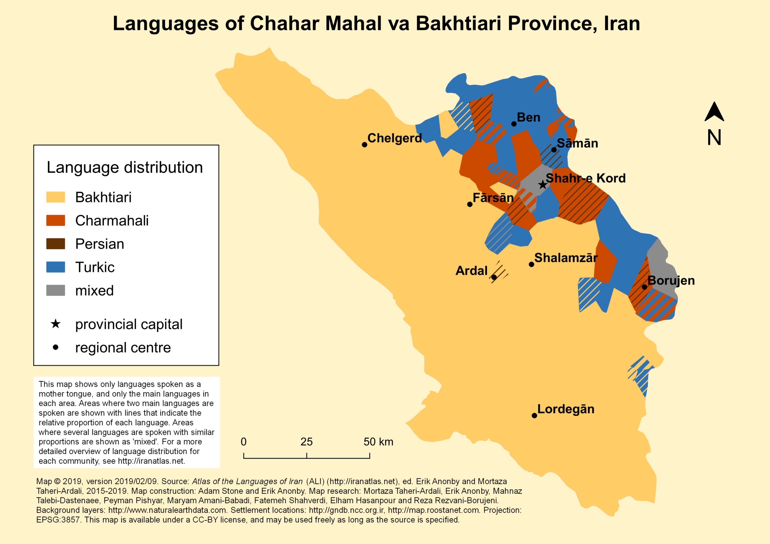


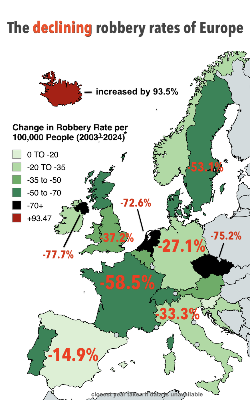

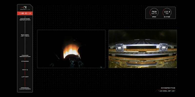


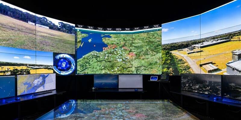
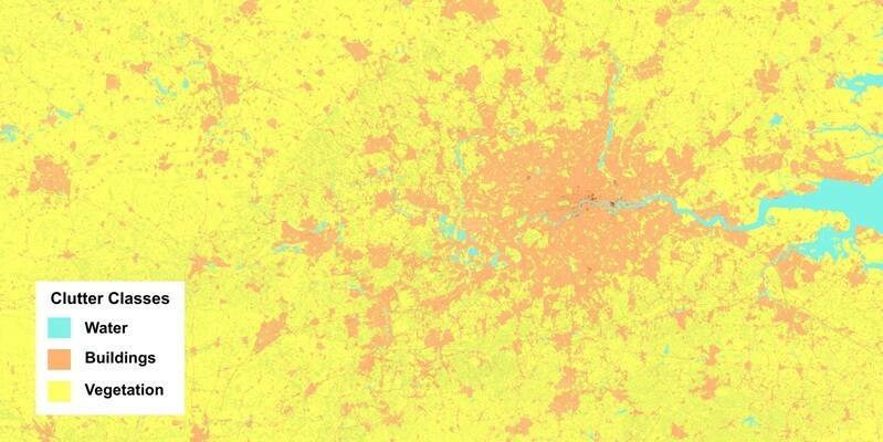


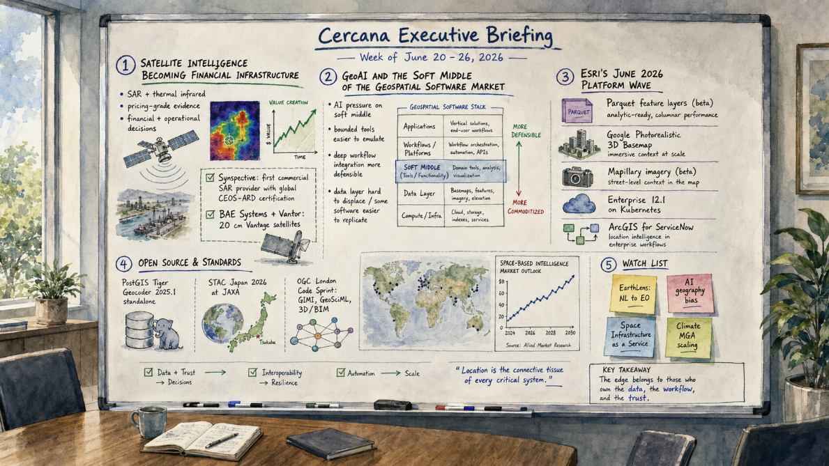

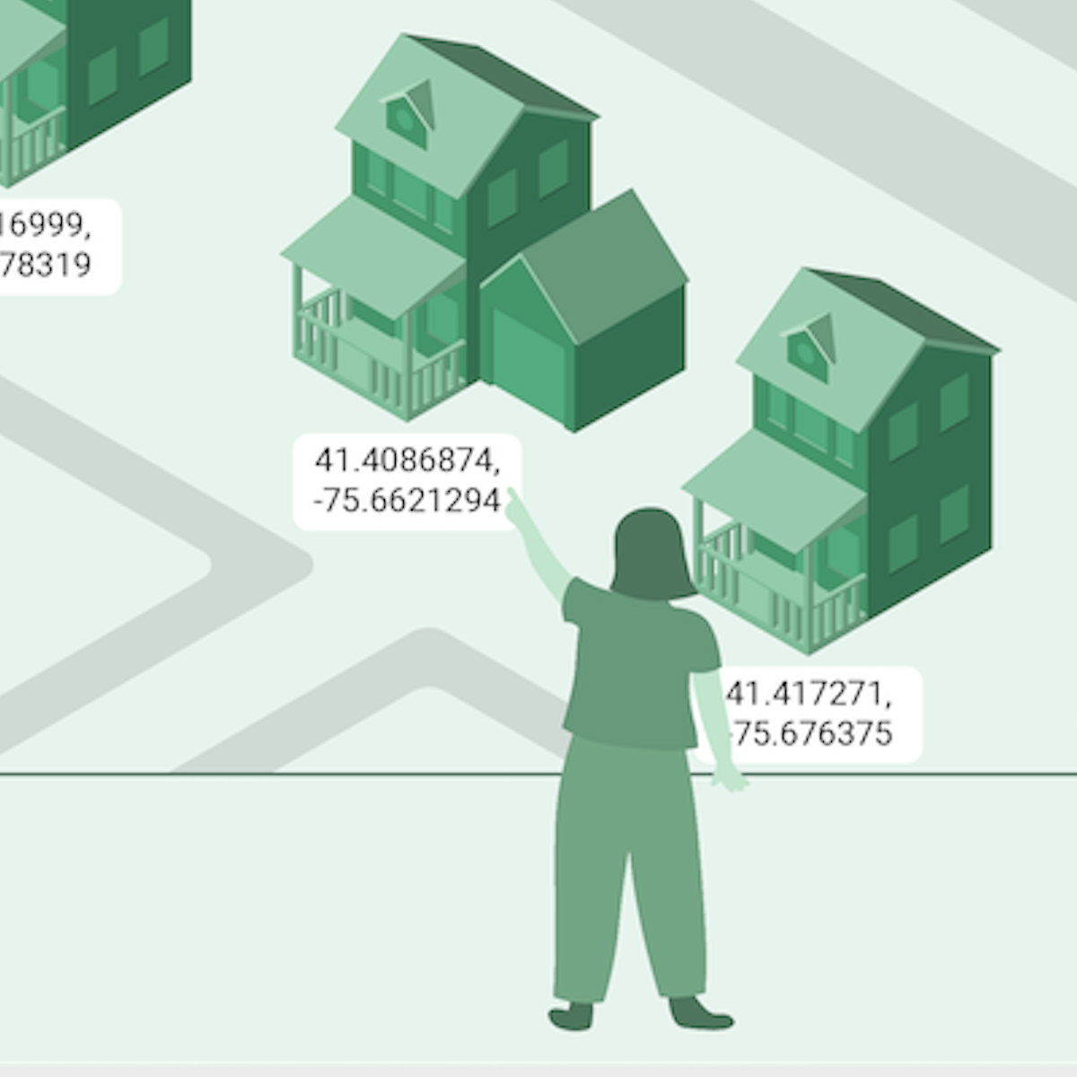


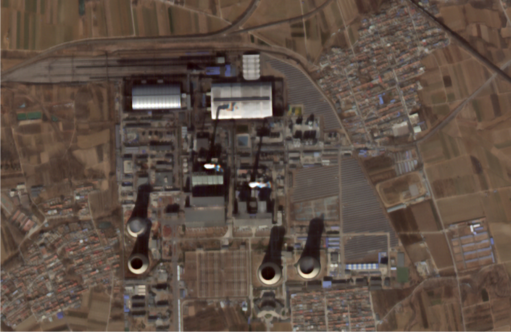
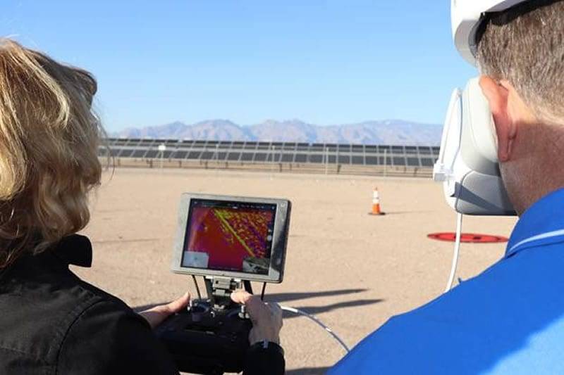


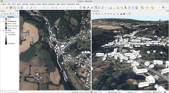
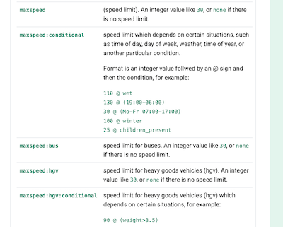

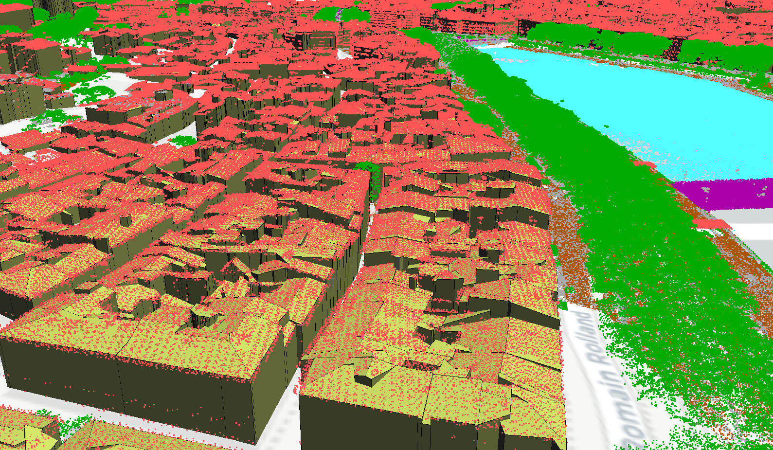


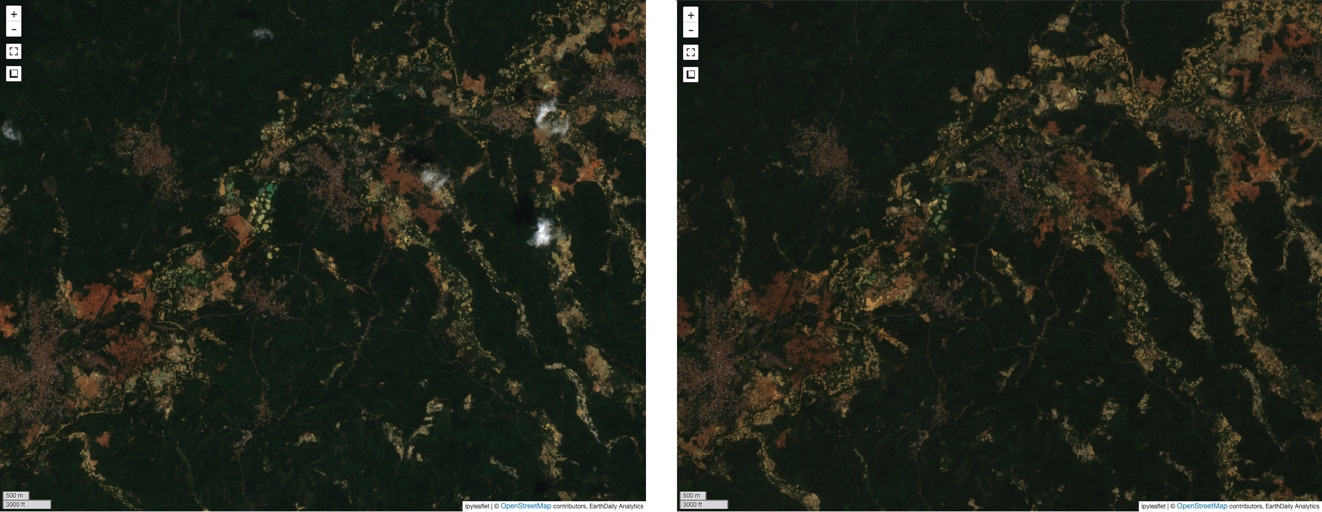
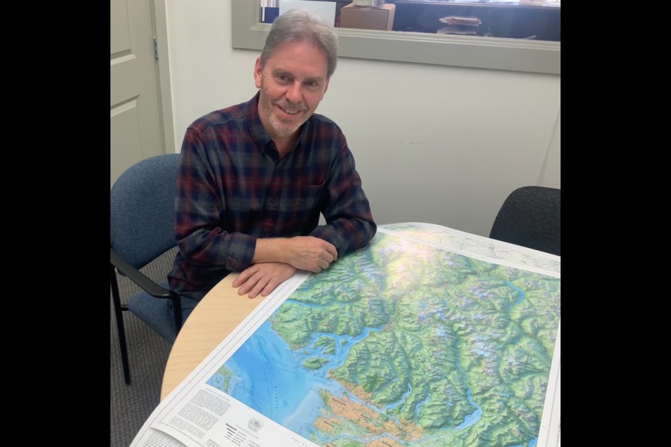
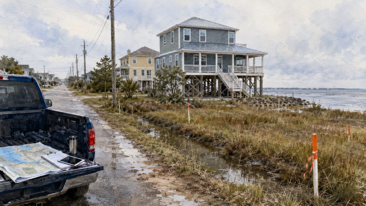


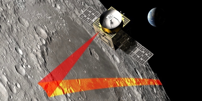
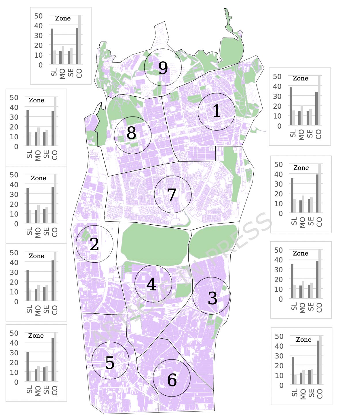


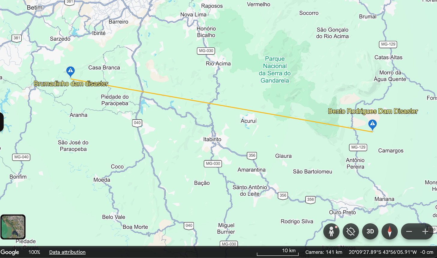

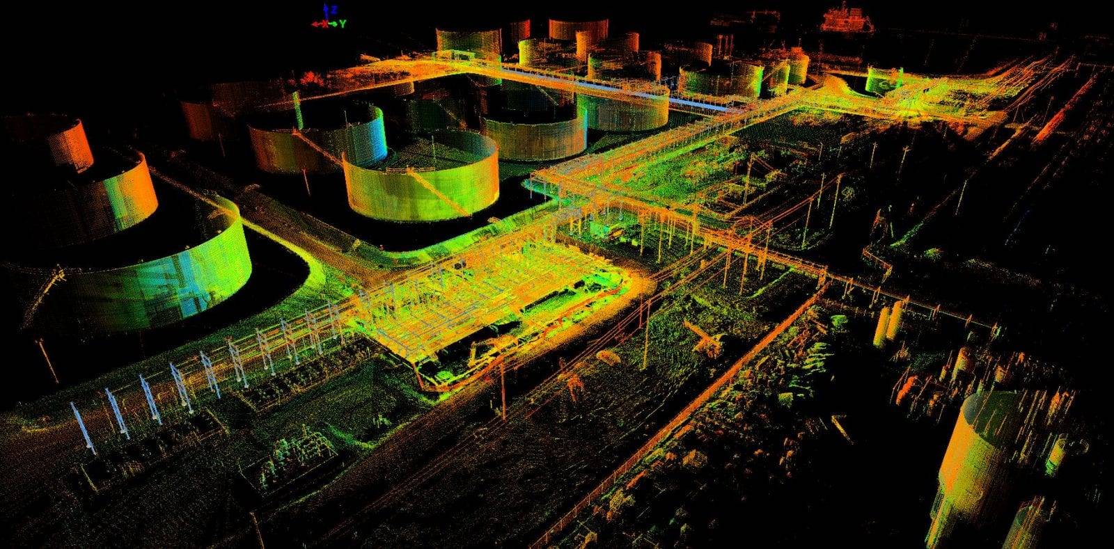
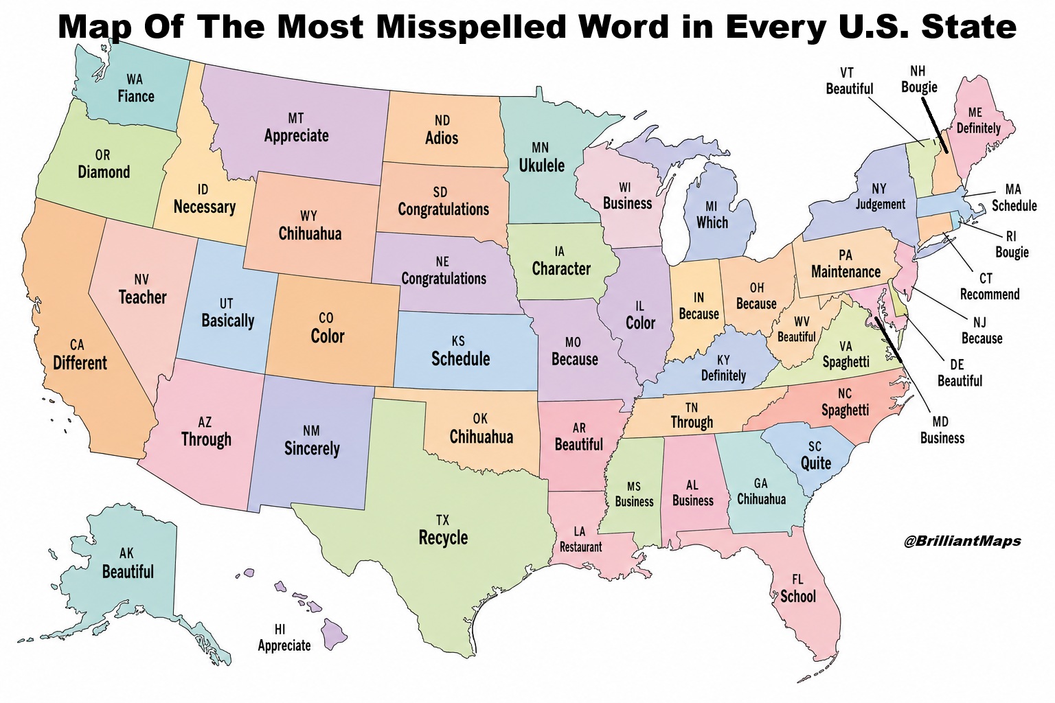
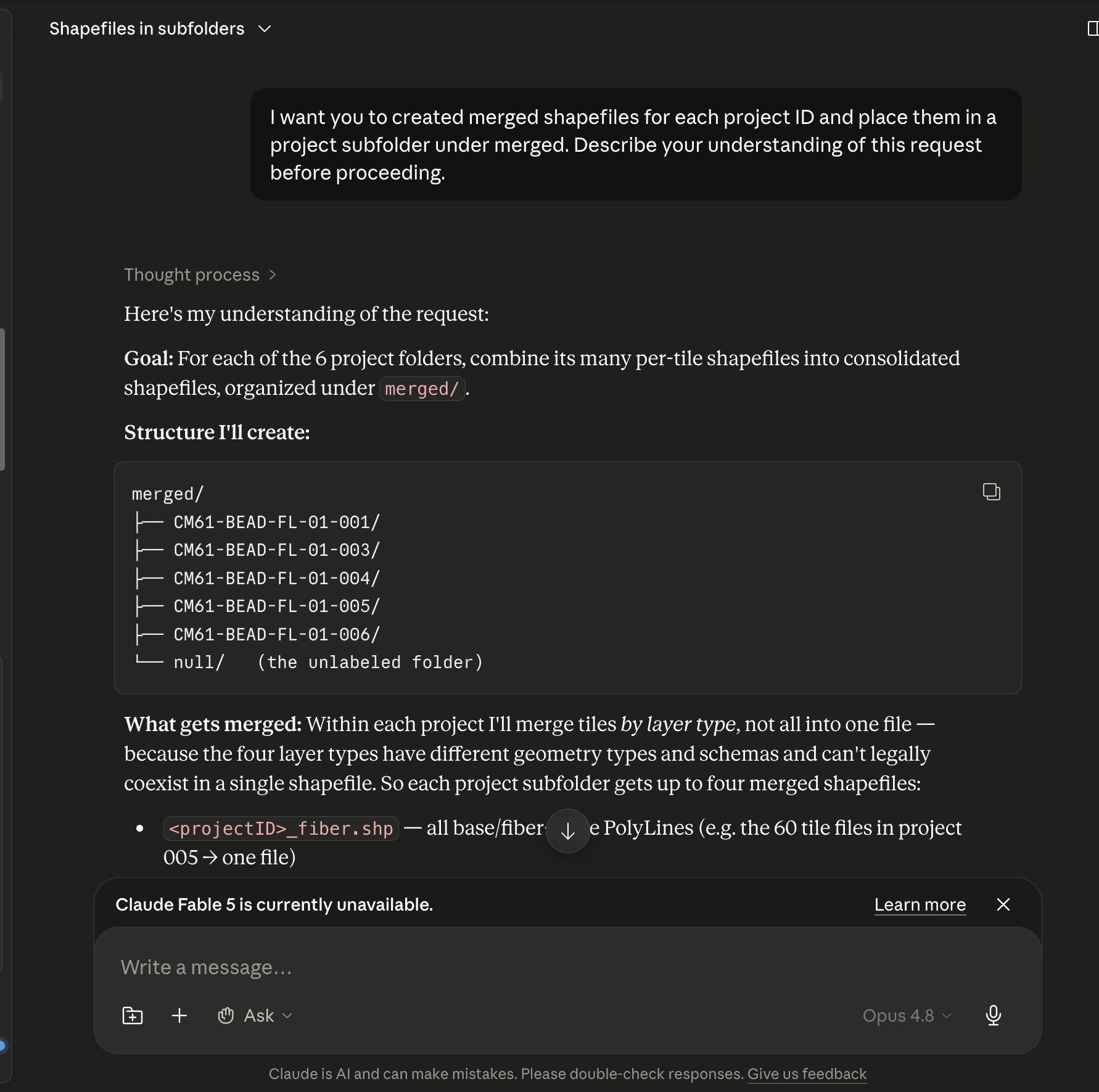


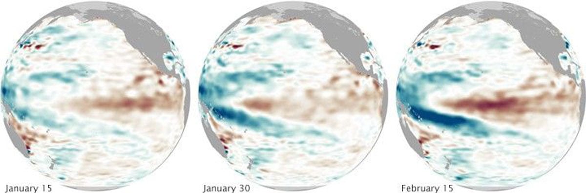

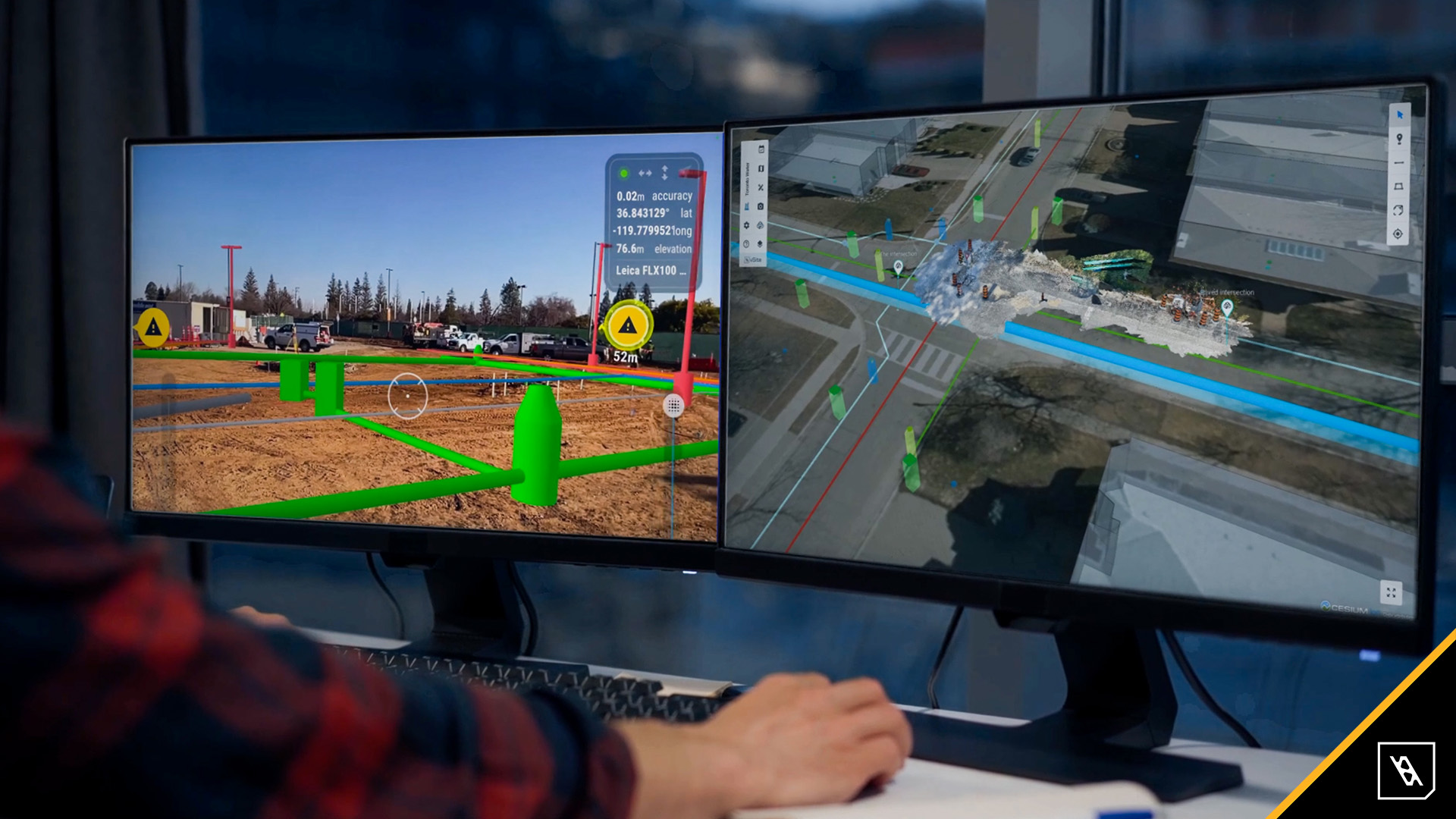

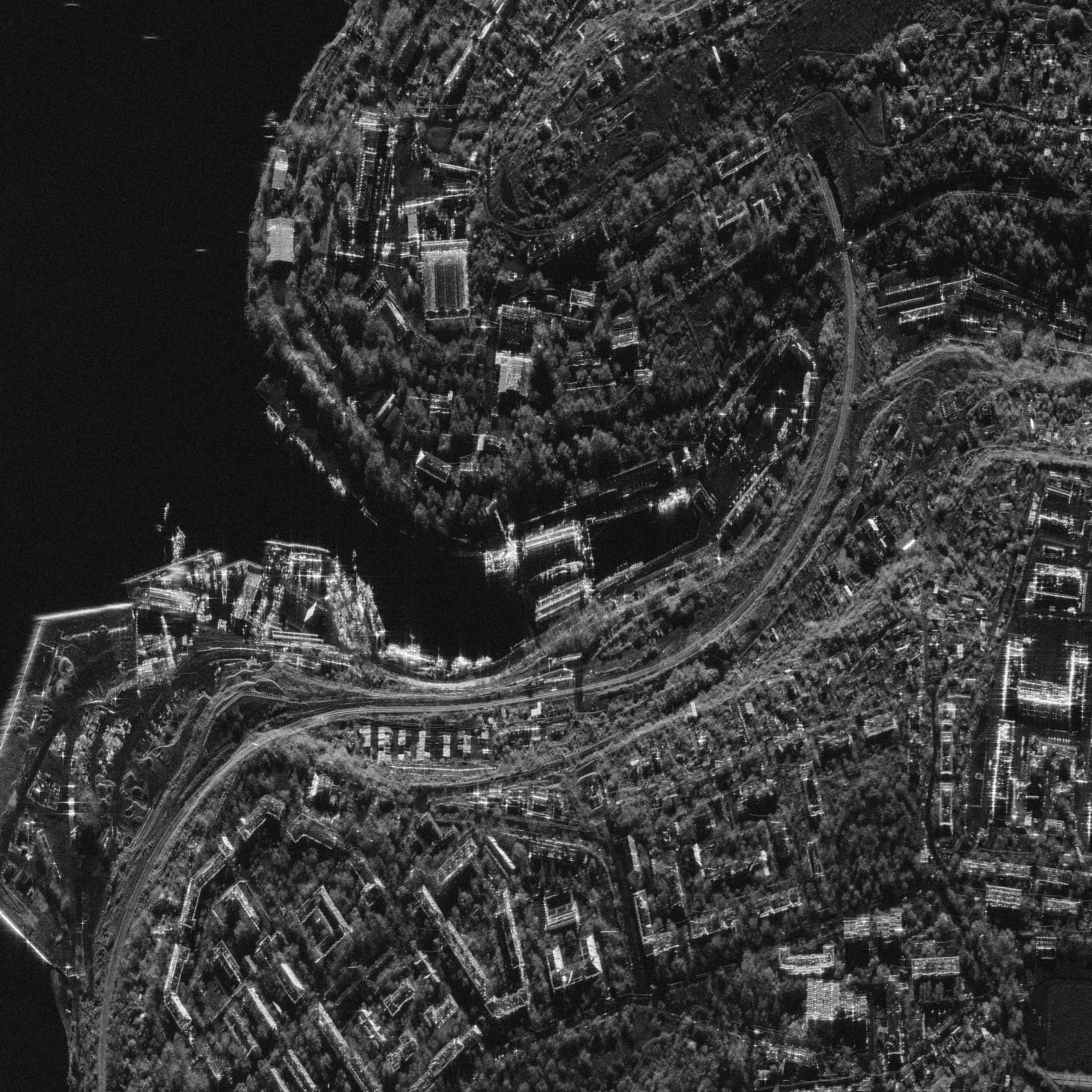

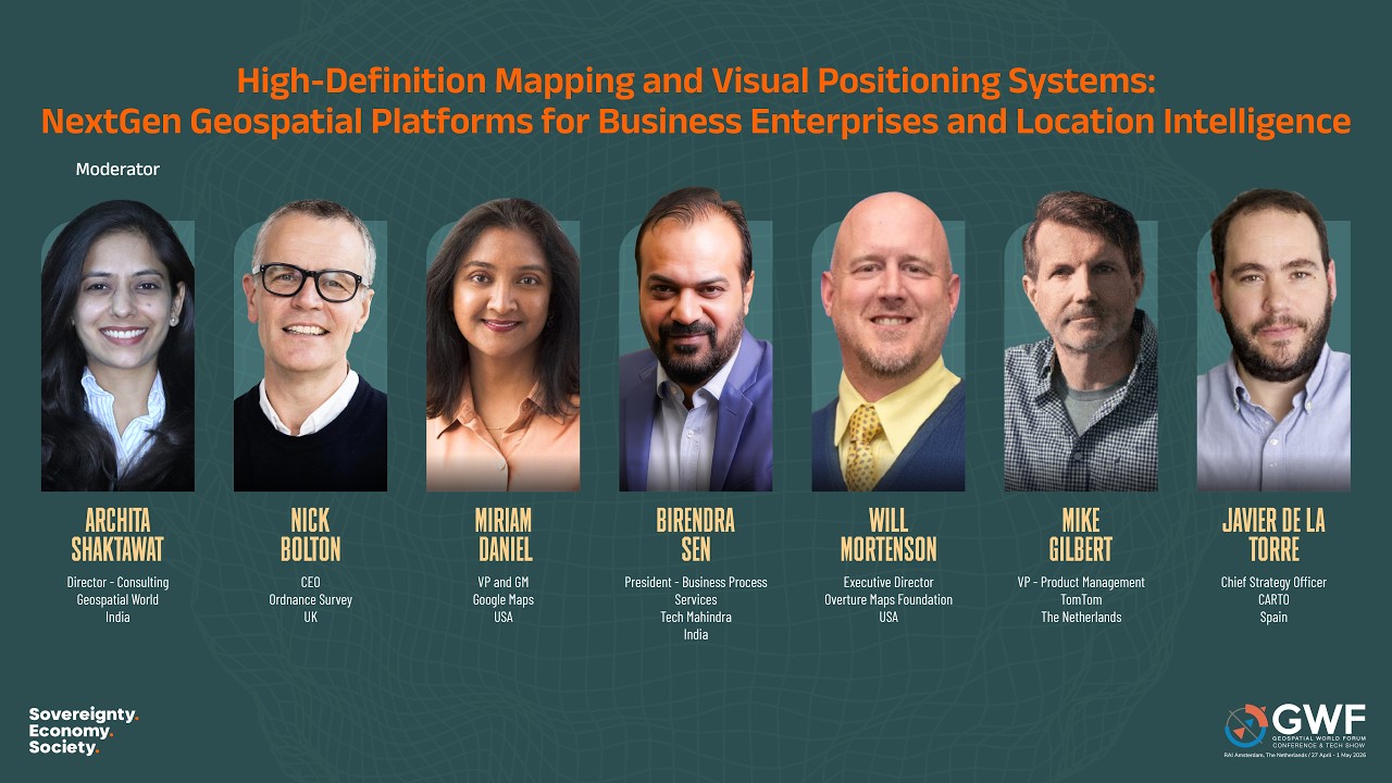
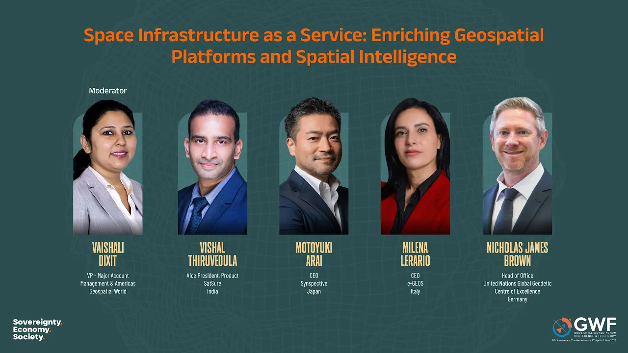


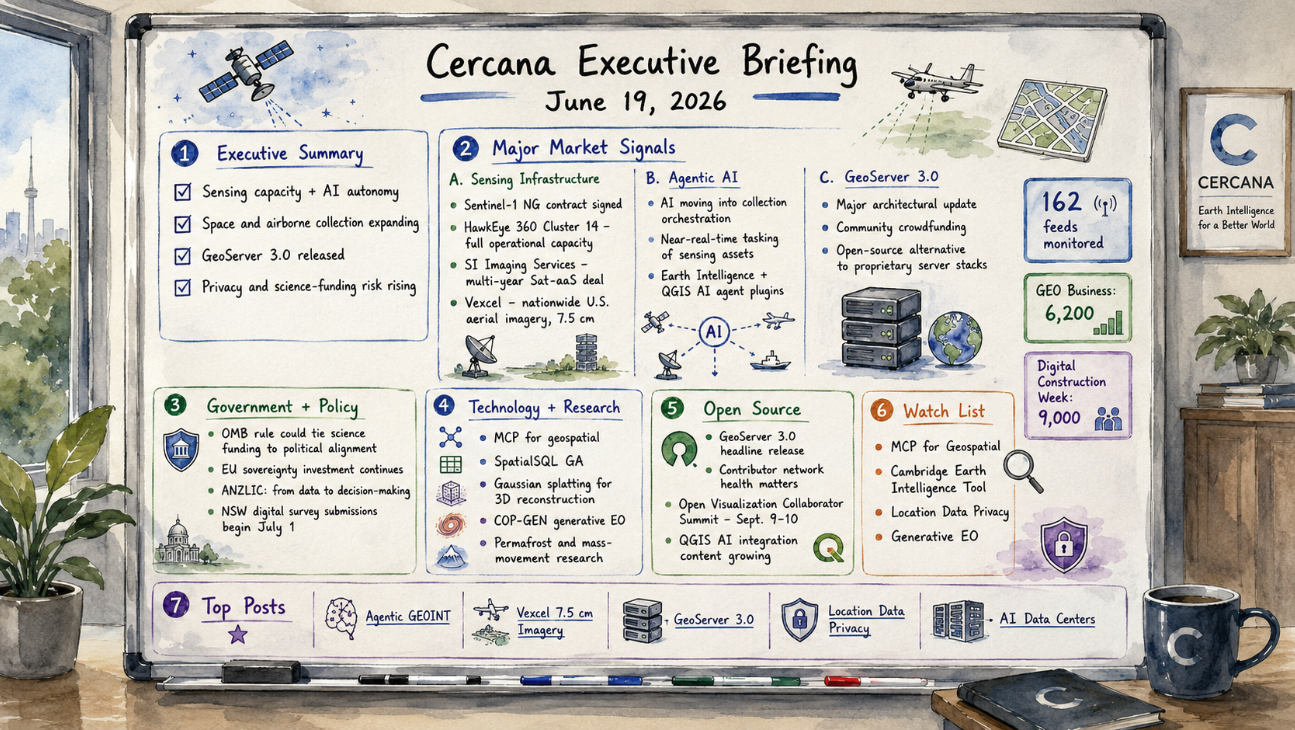


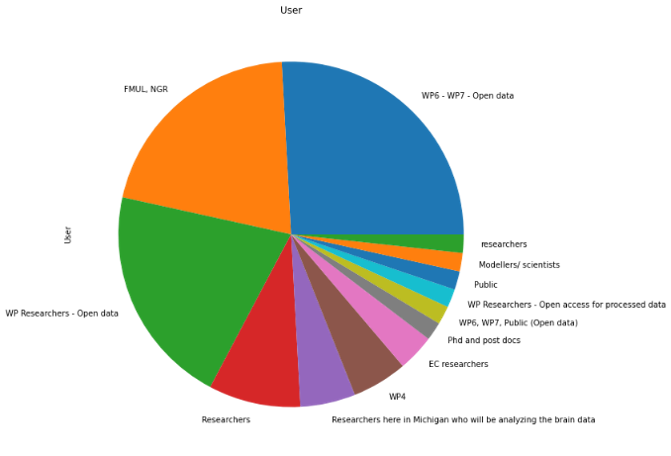
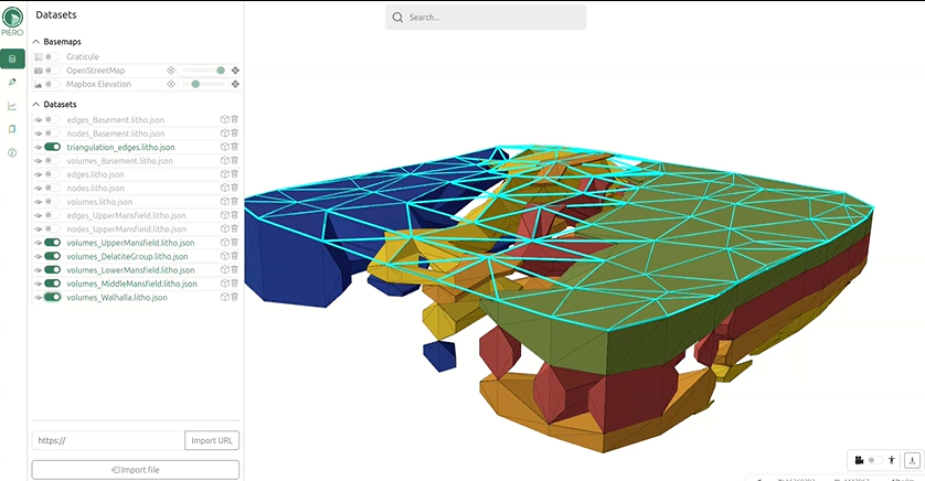
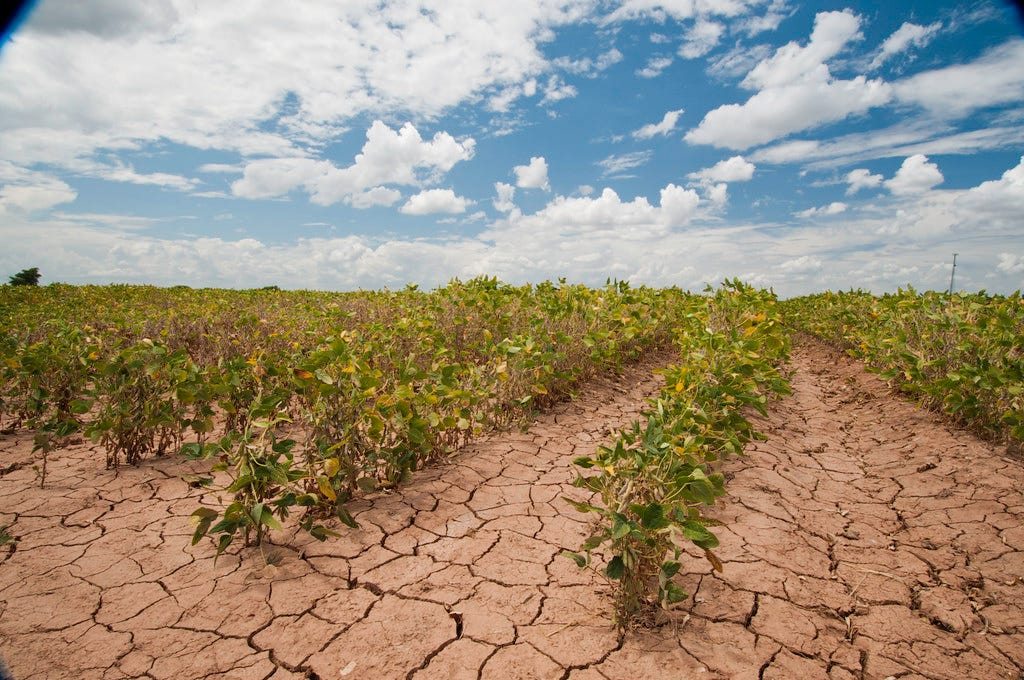


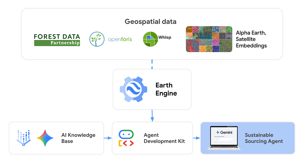


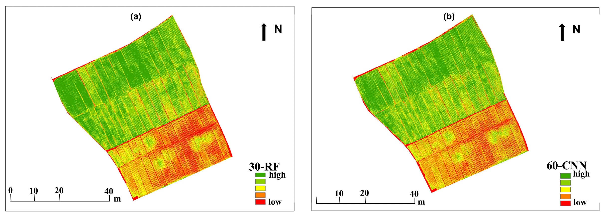
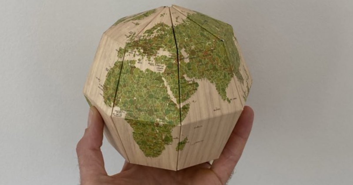
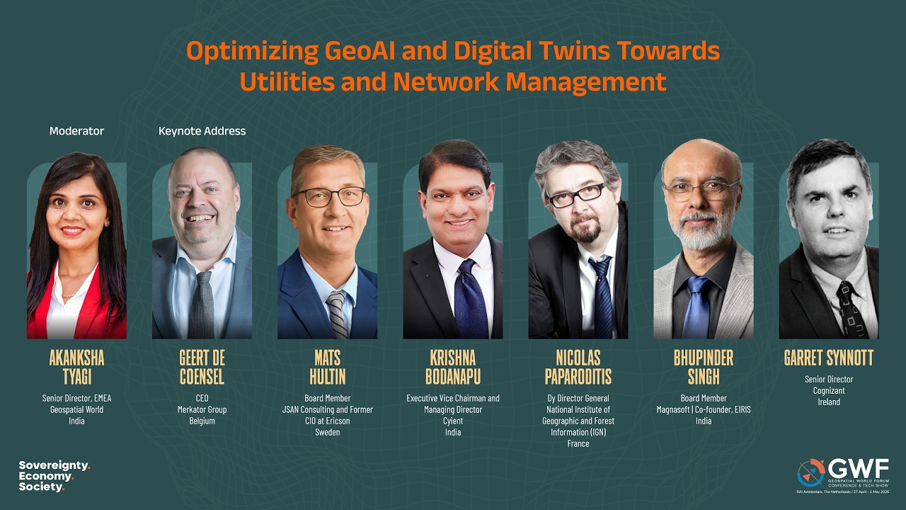


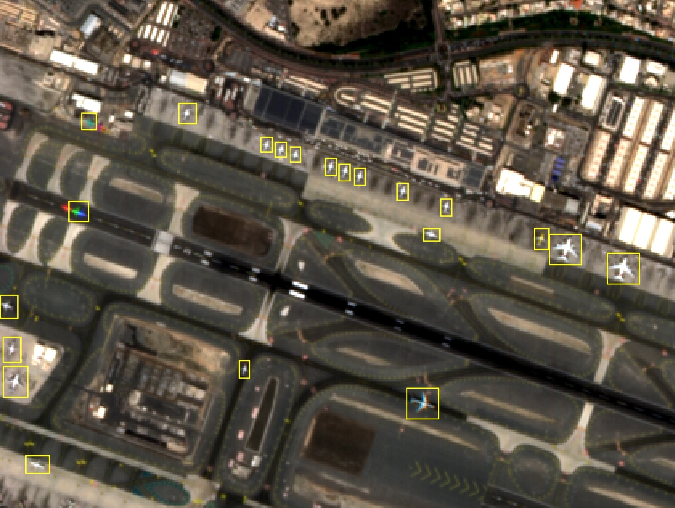


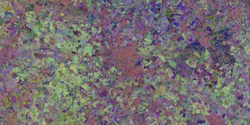
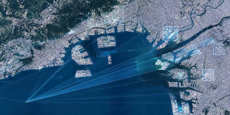


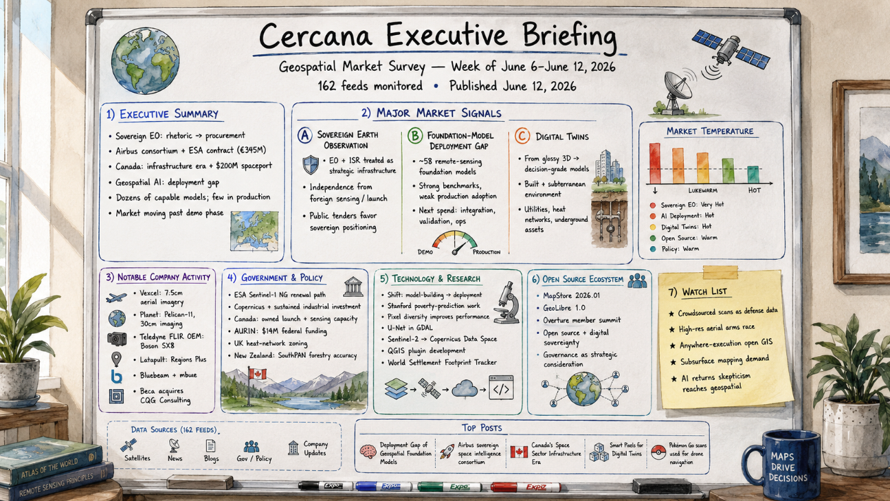
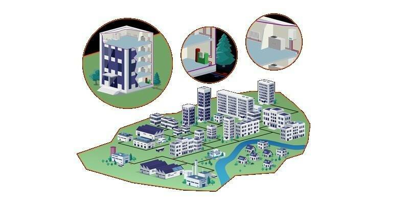

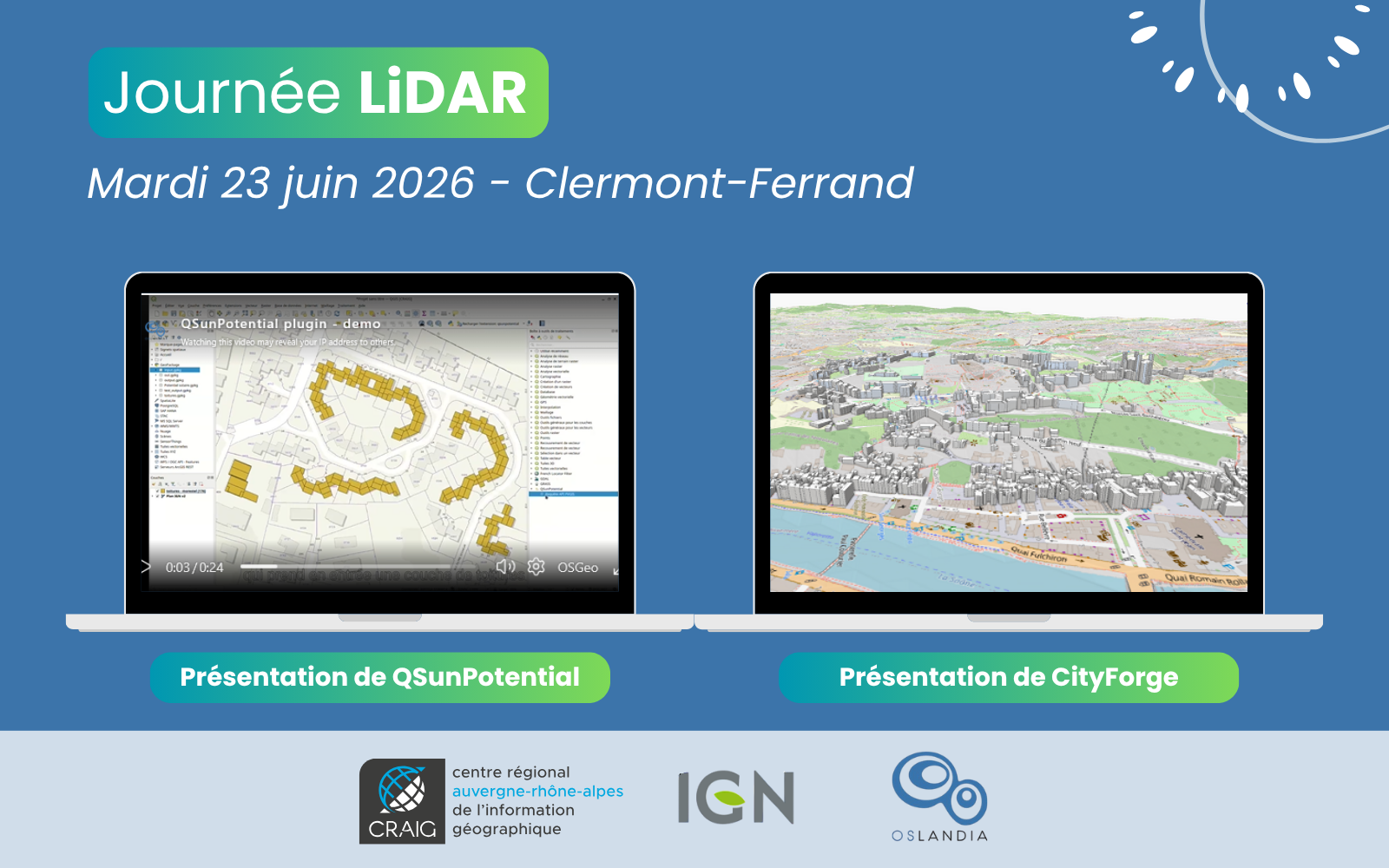
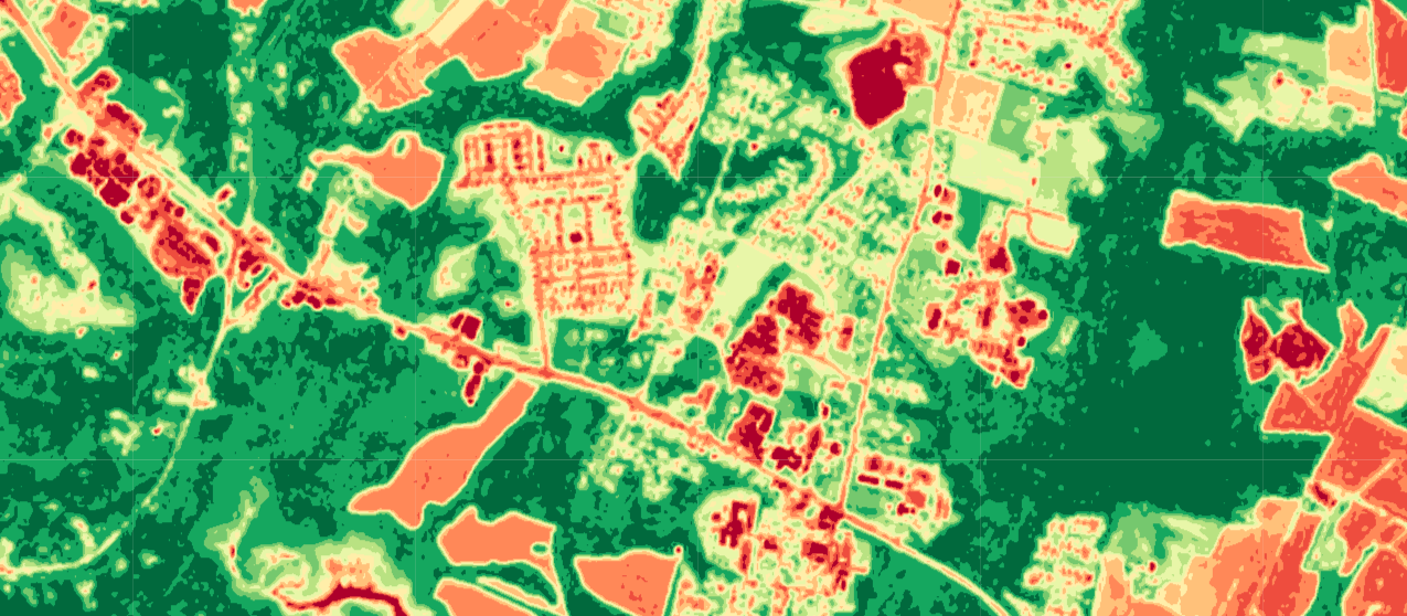


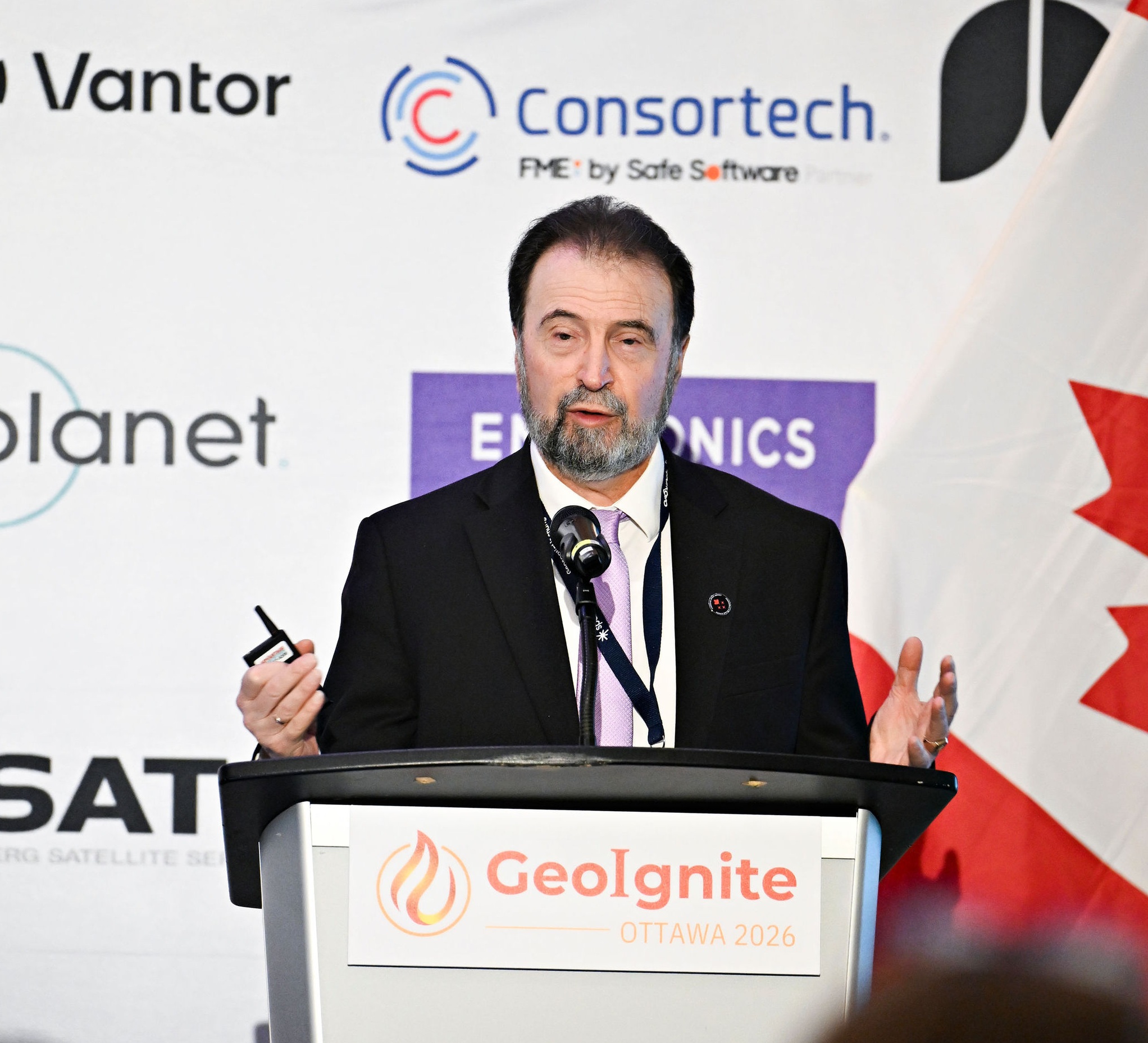
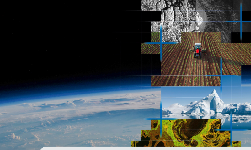
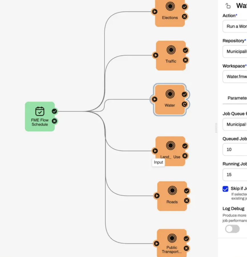
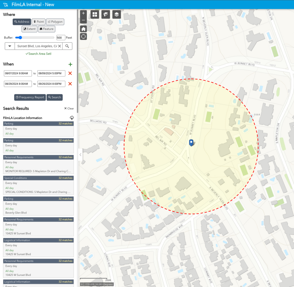


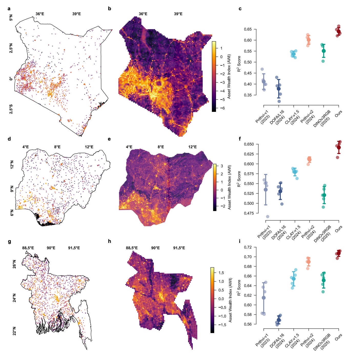


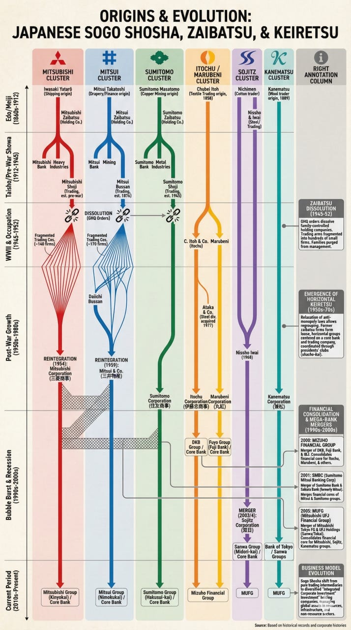
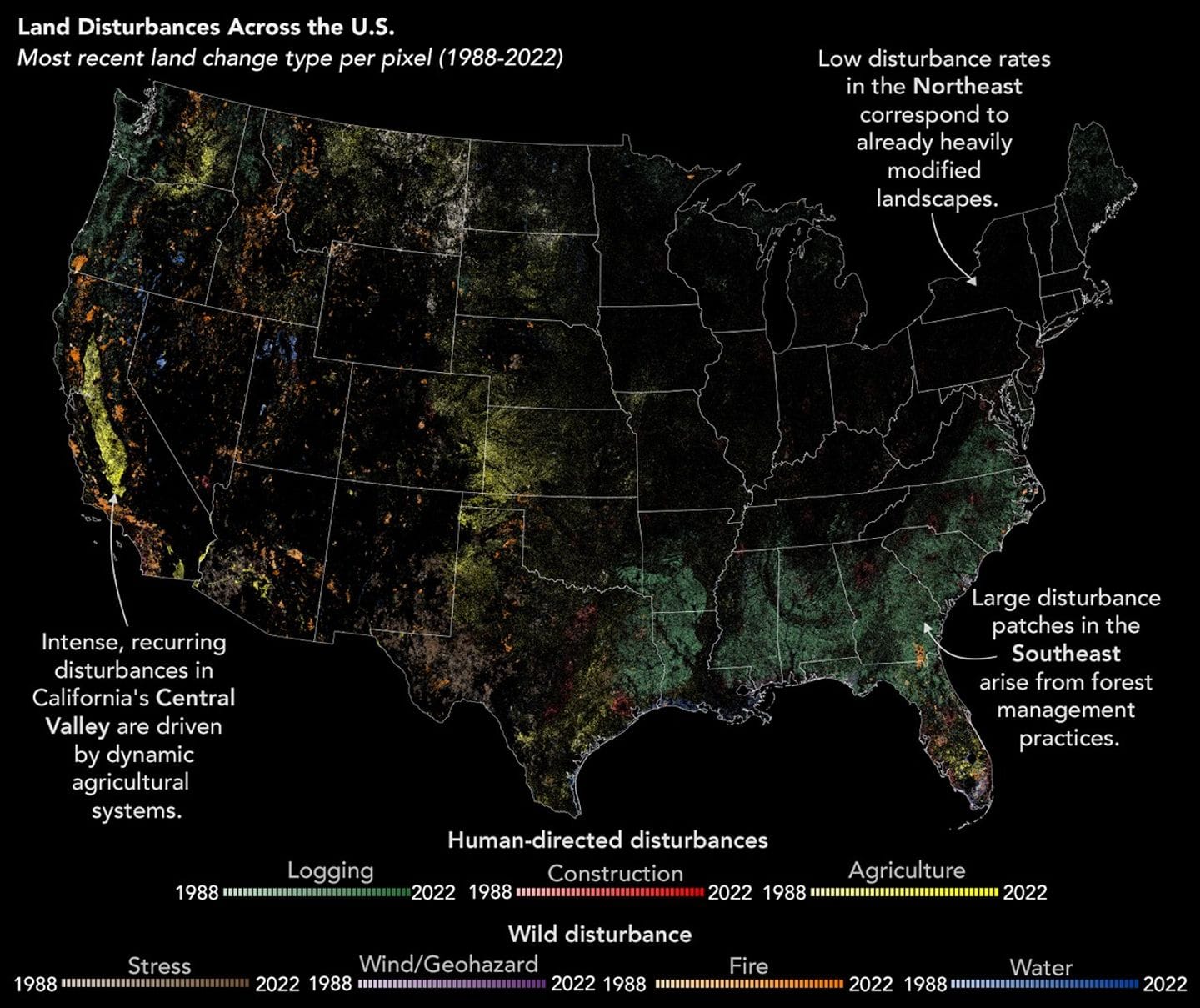


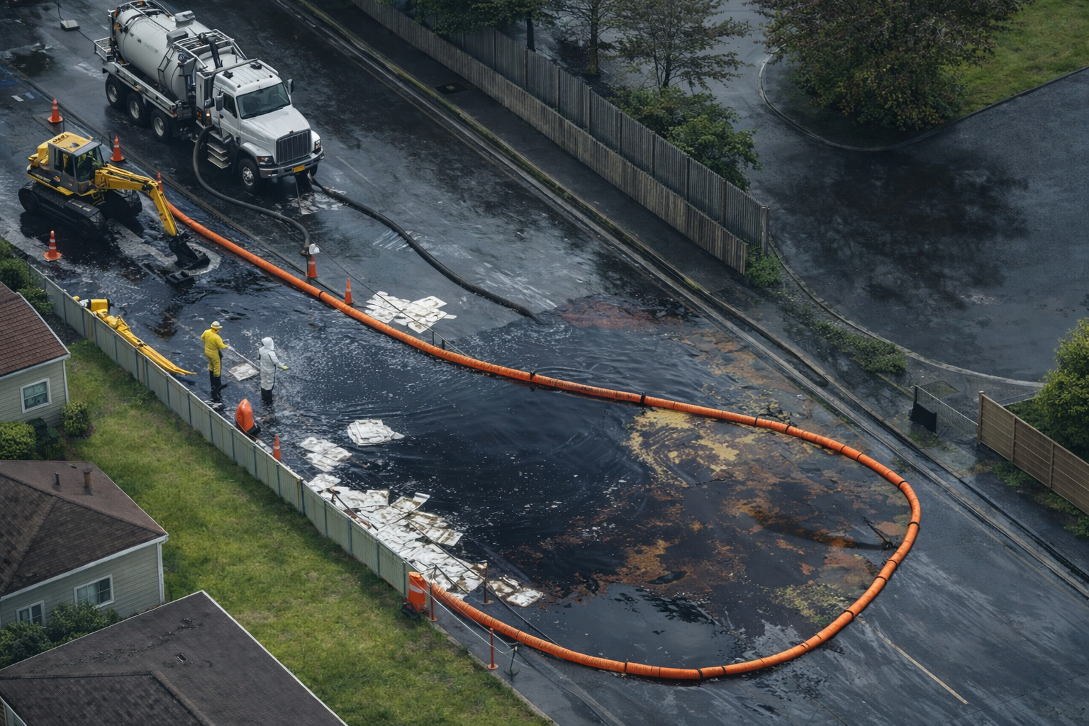


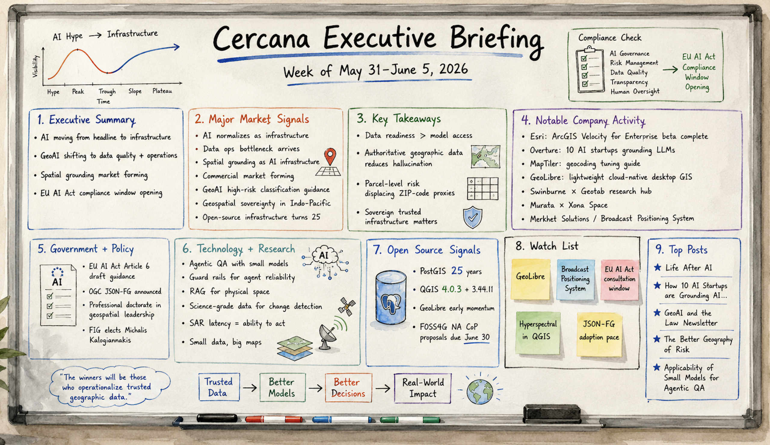

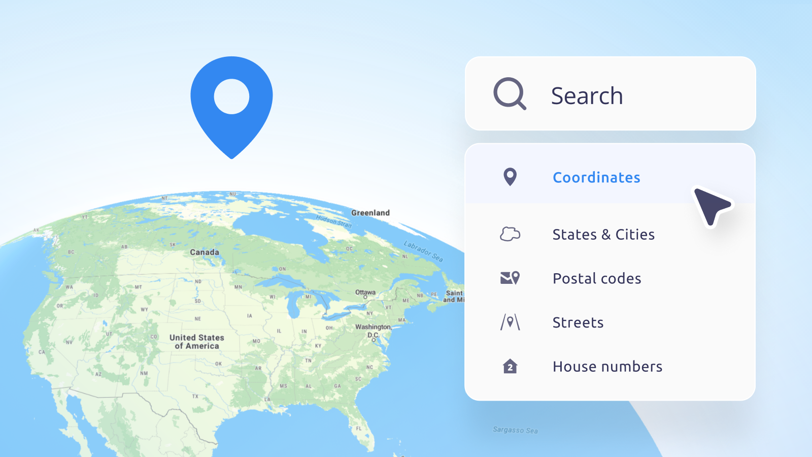
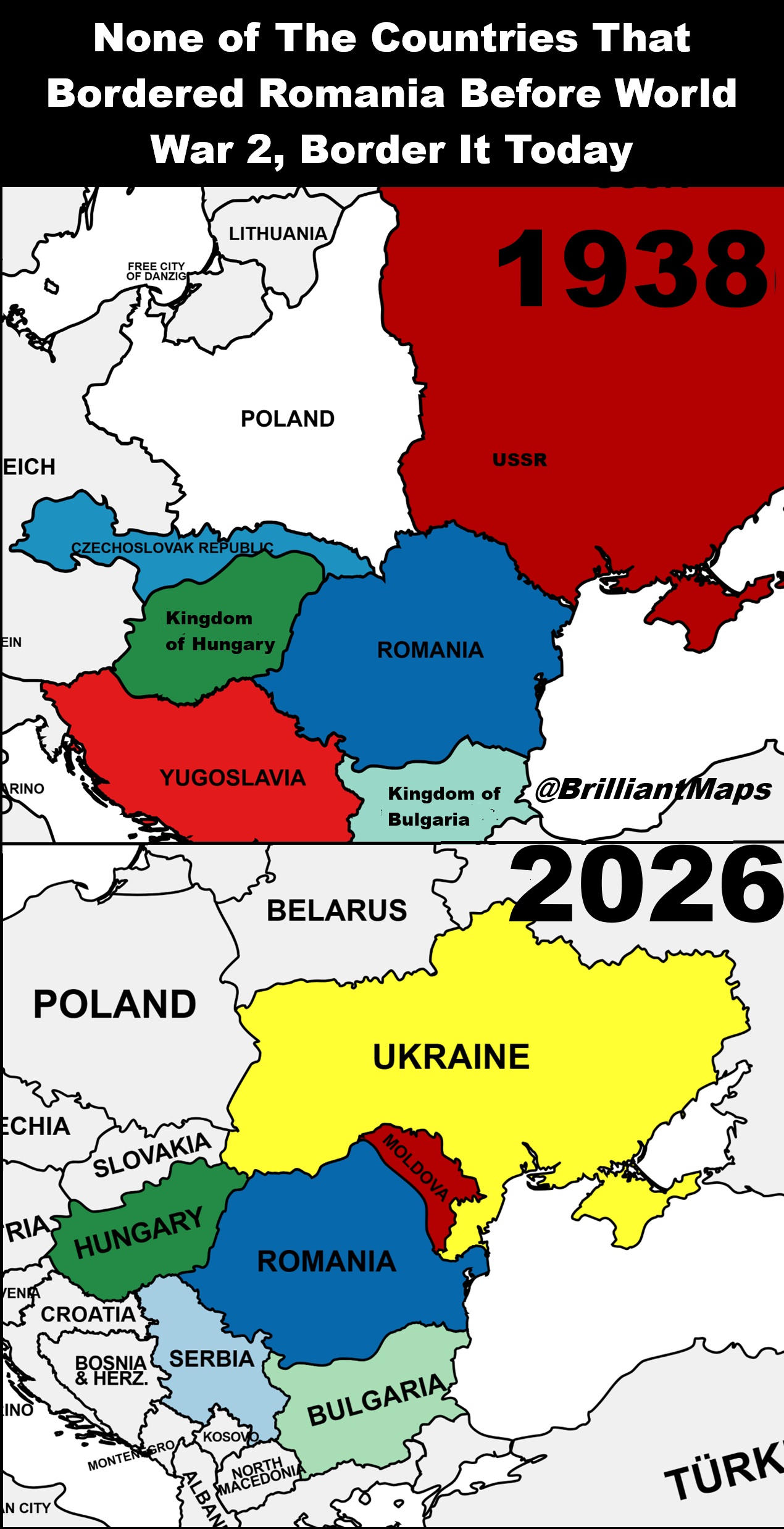


![Oslandia - [Webinar / discussion panel] Creating QGIS plugins in 2026](https://oslandia.com/wp-content/uploads/2026/06/webinar-plugins-QGIS-oslandia-EN.png)

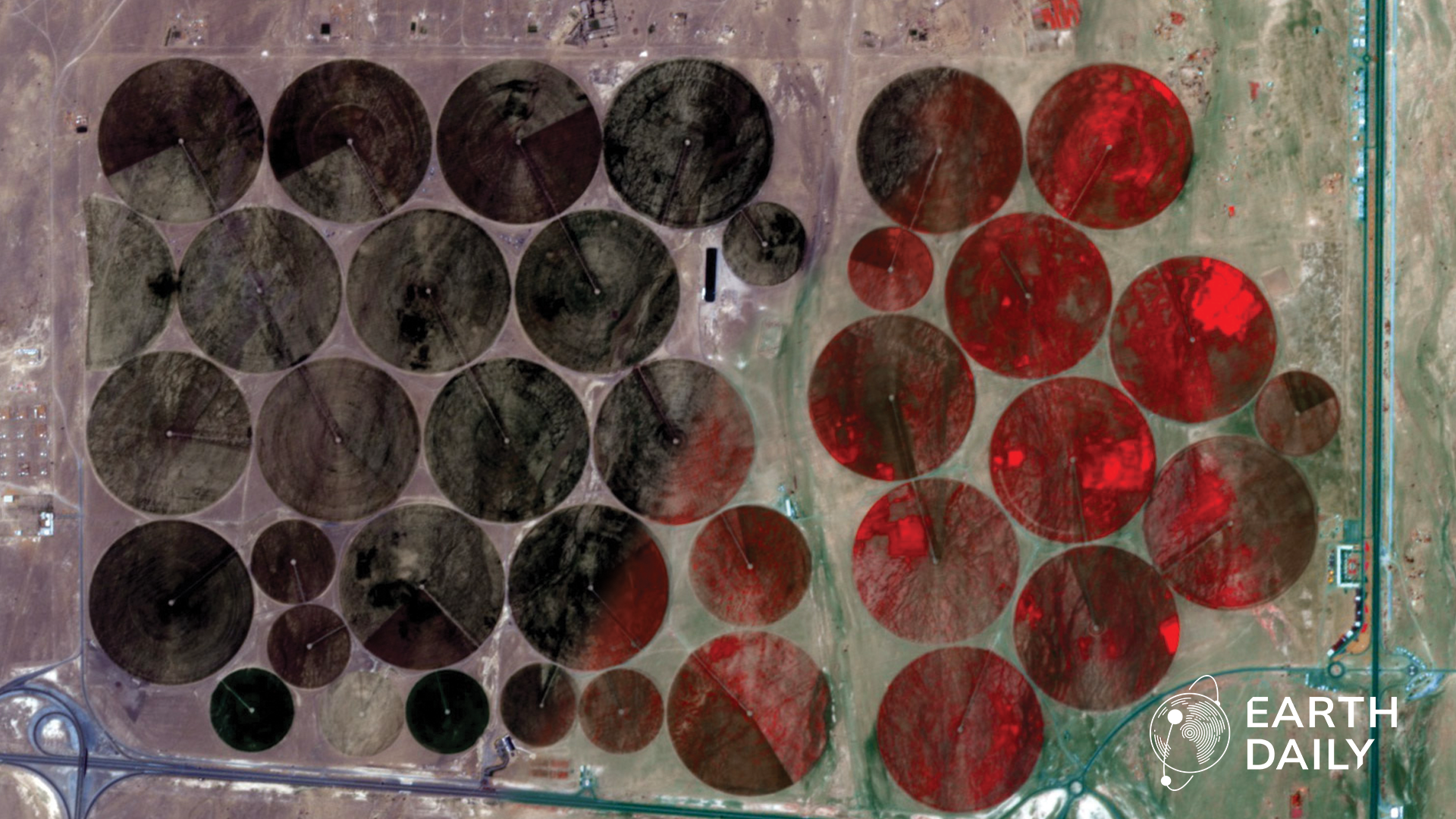
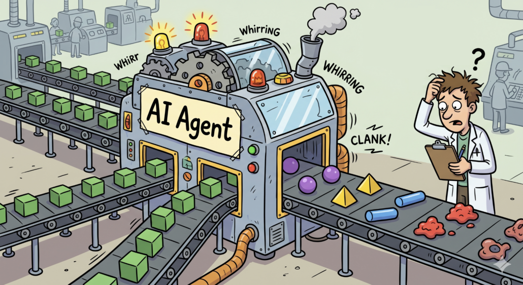

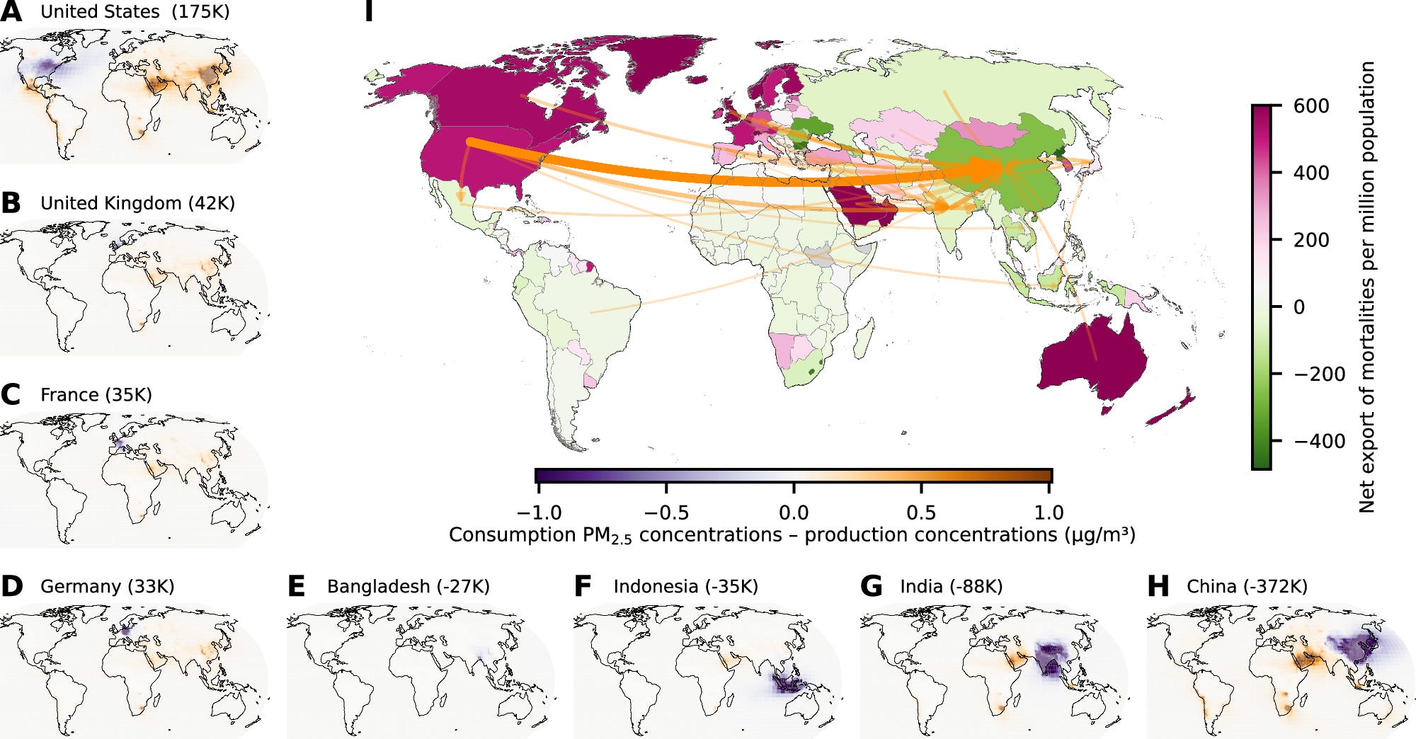

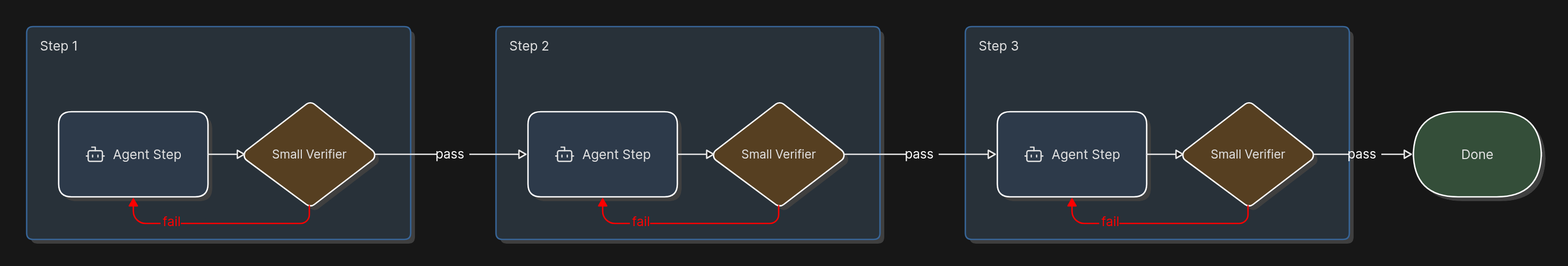
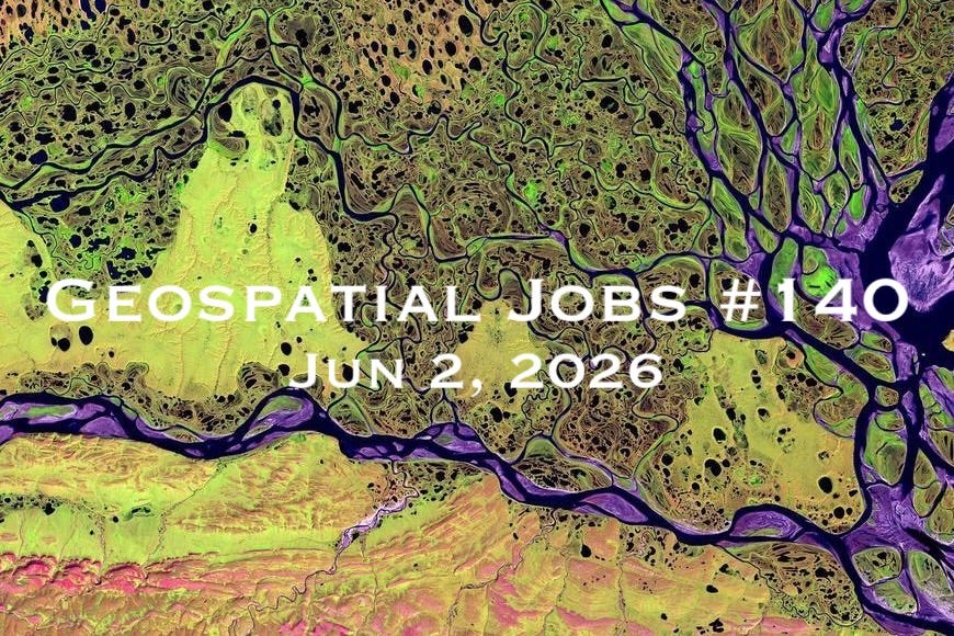
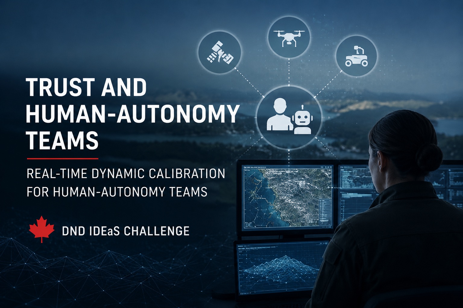

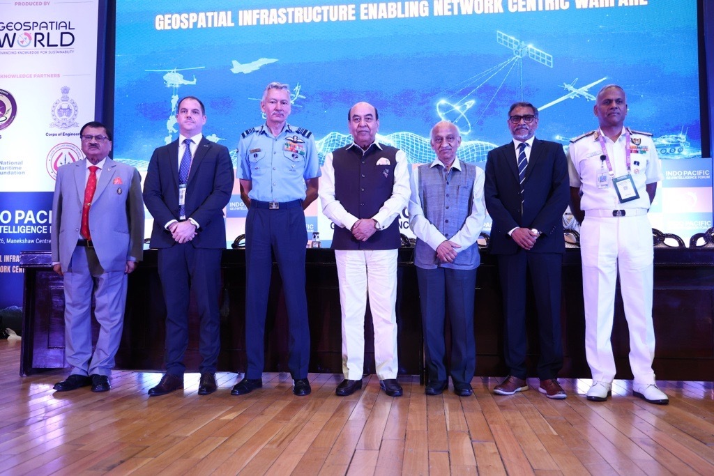
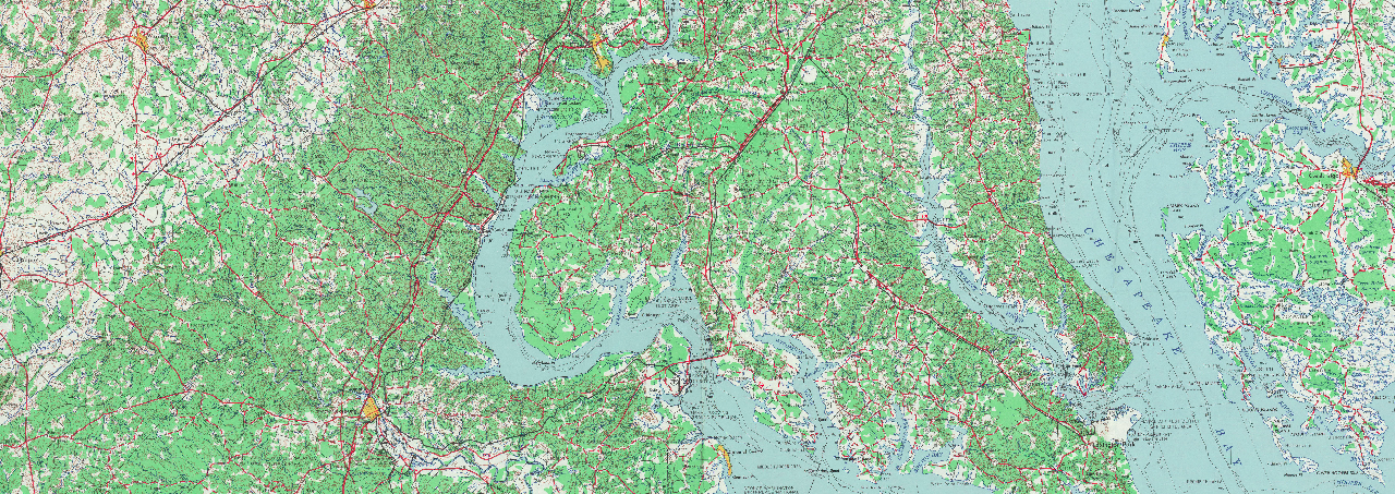
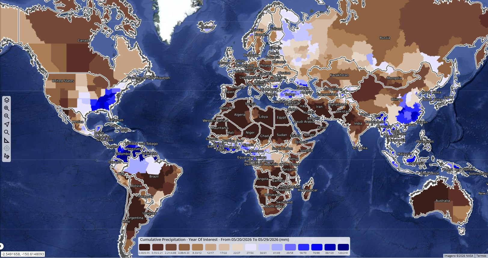


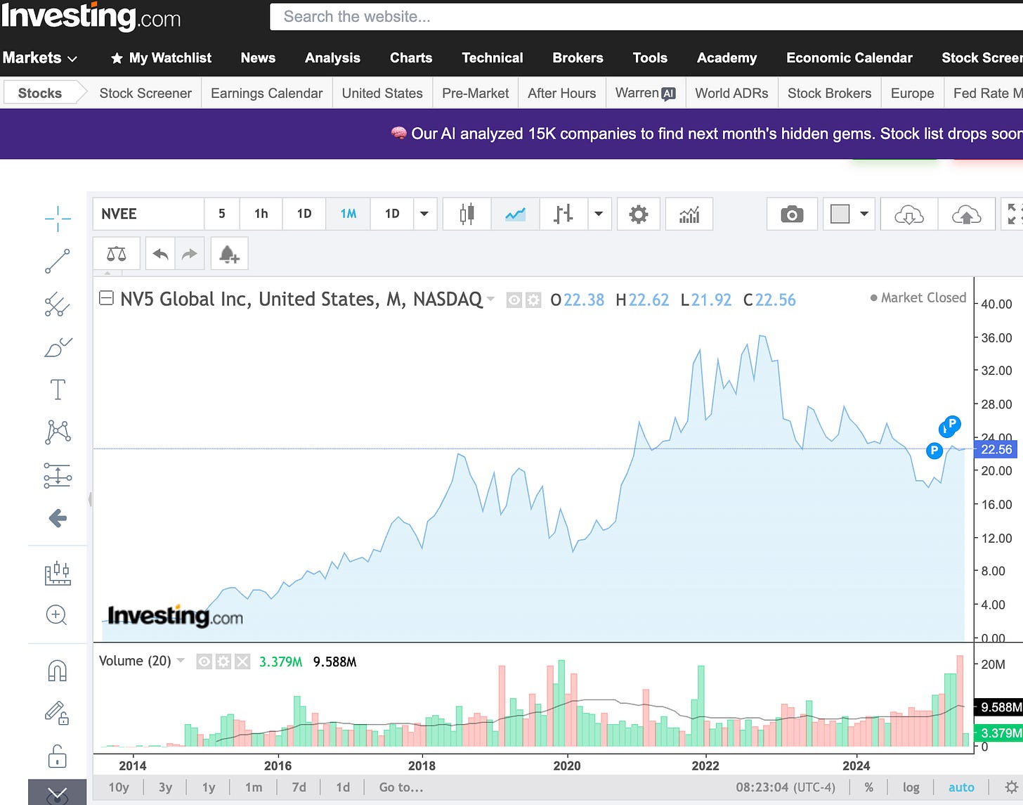


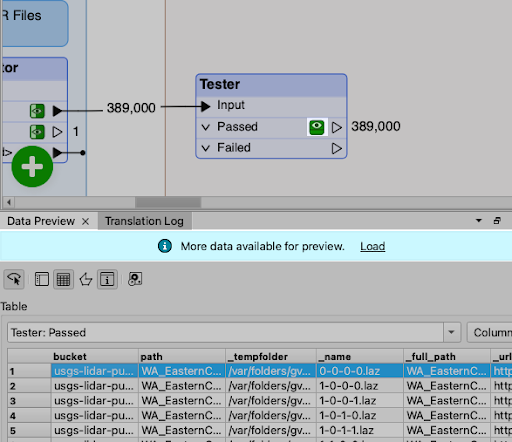

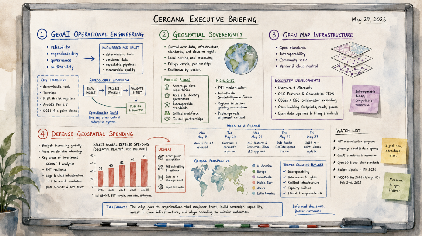

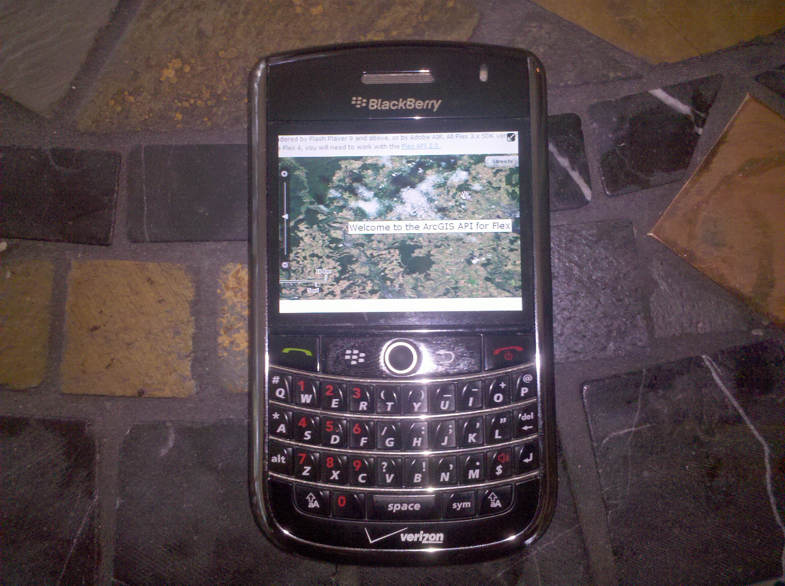


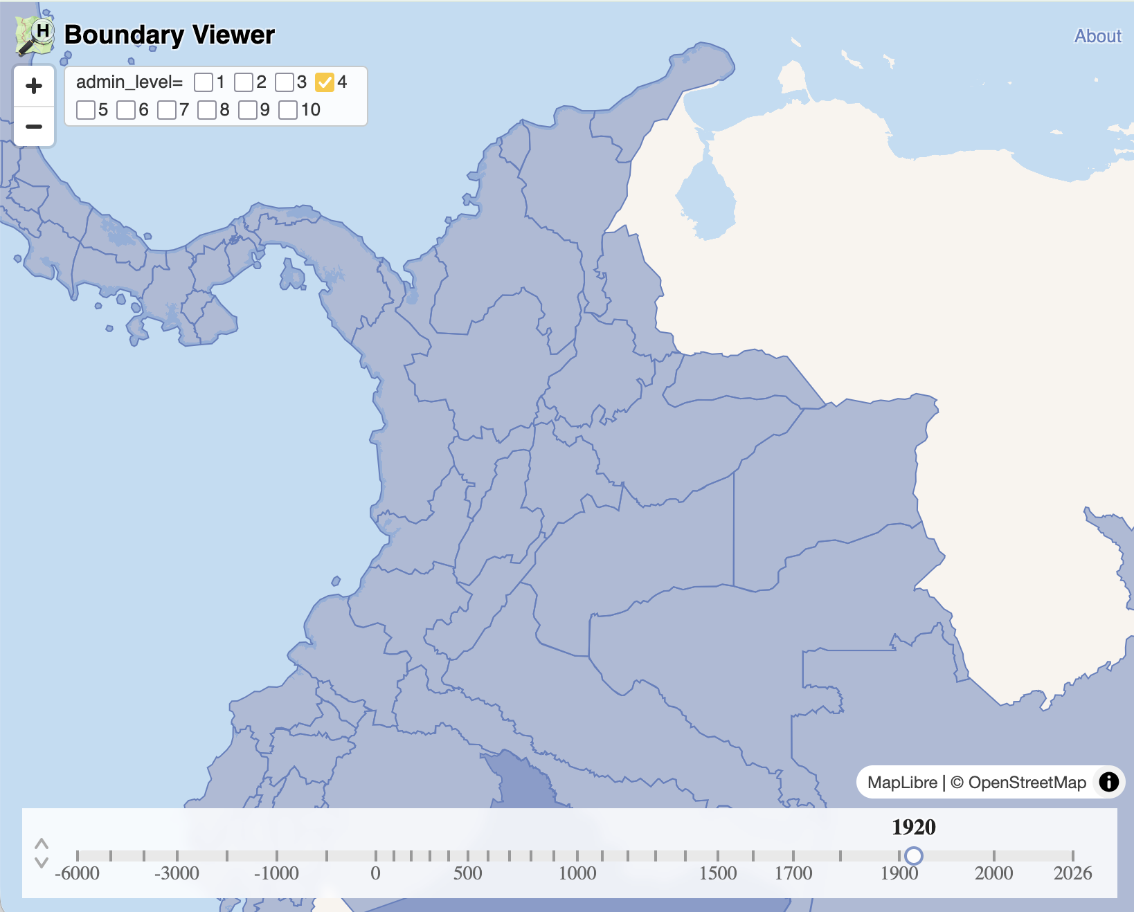


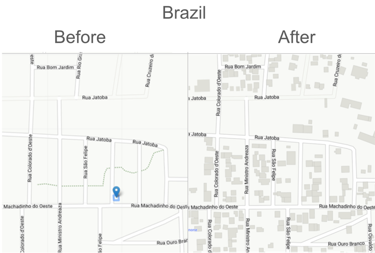
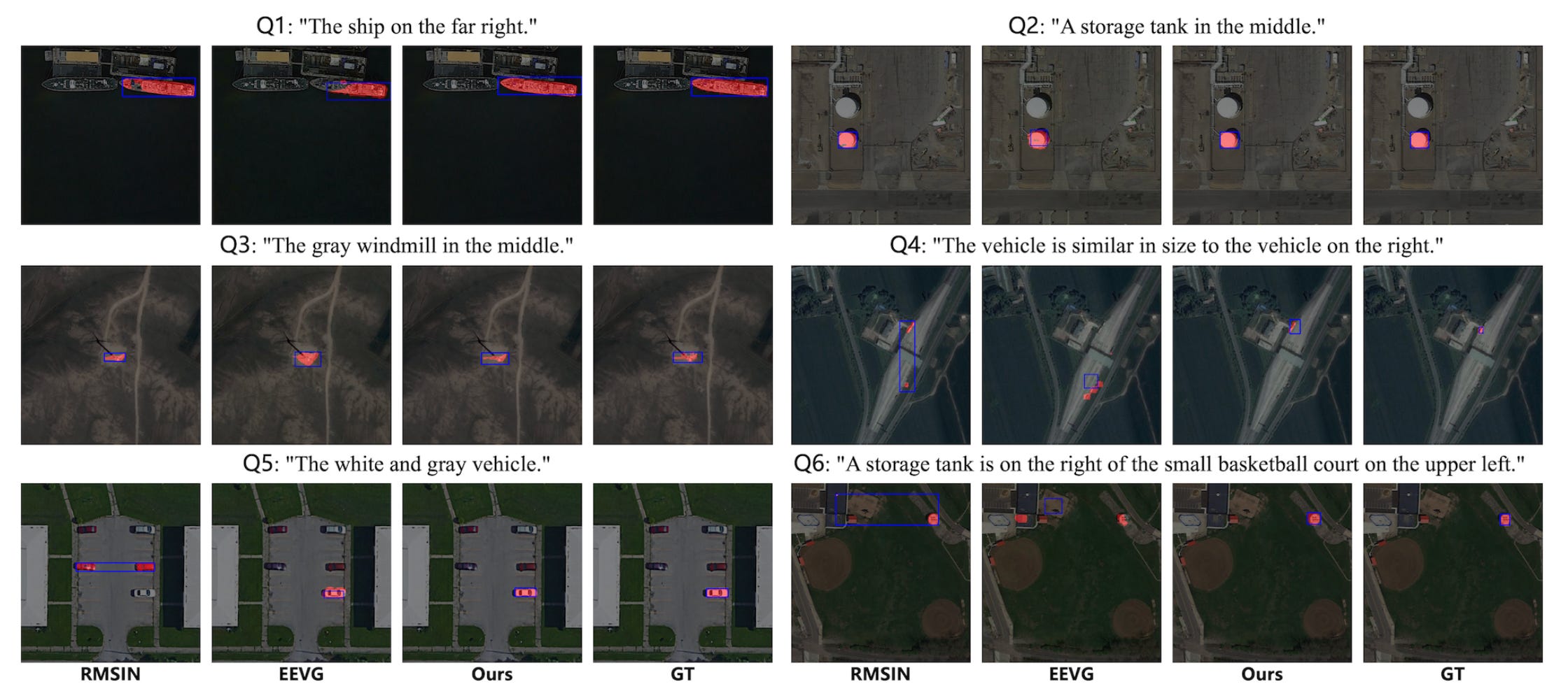
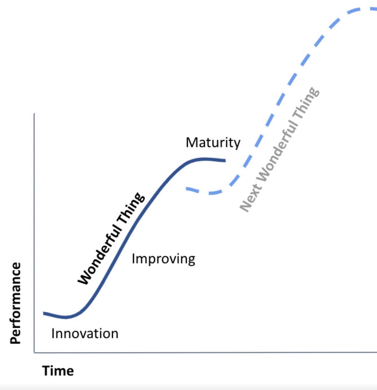

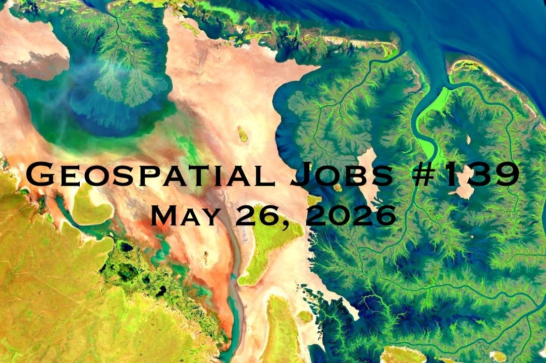

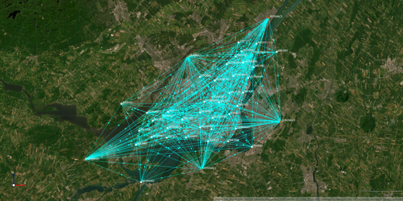


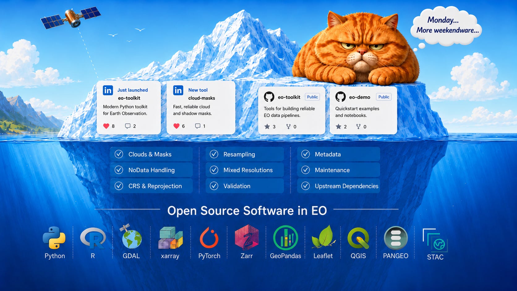


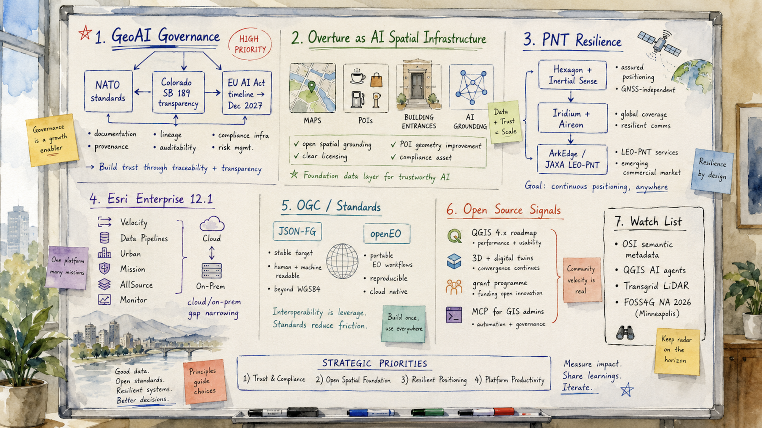


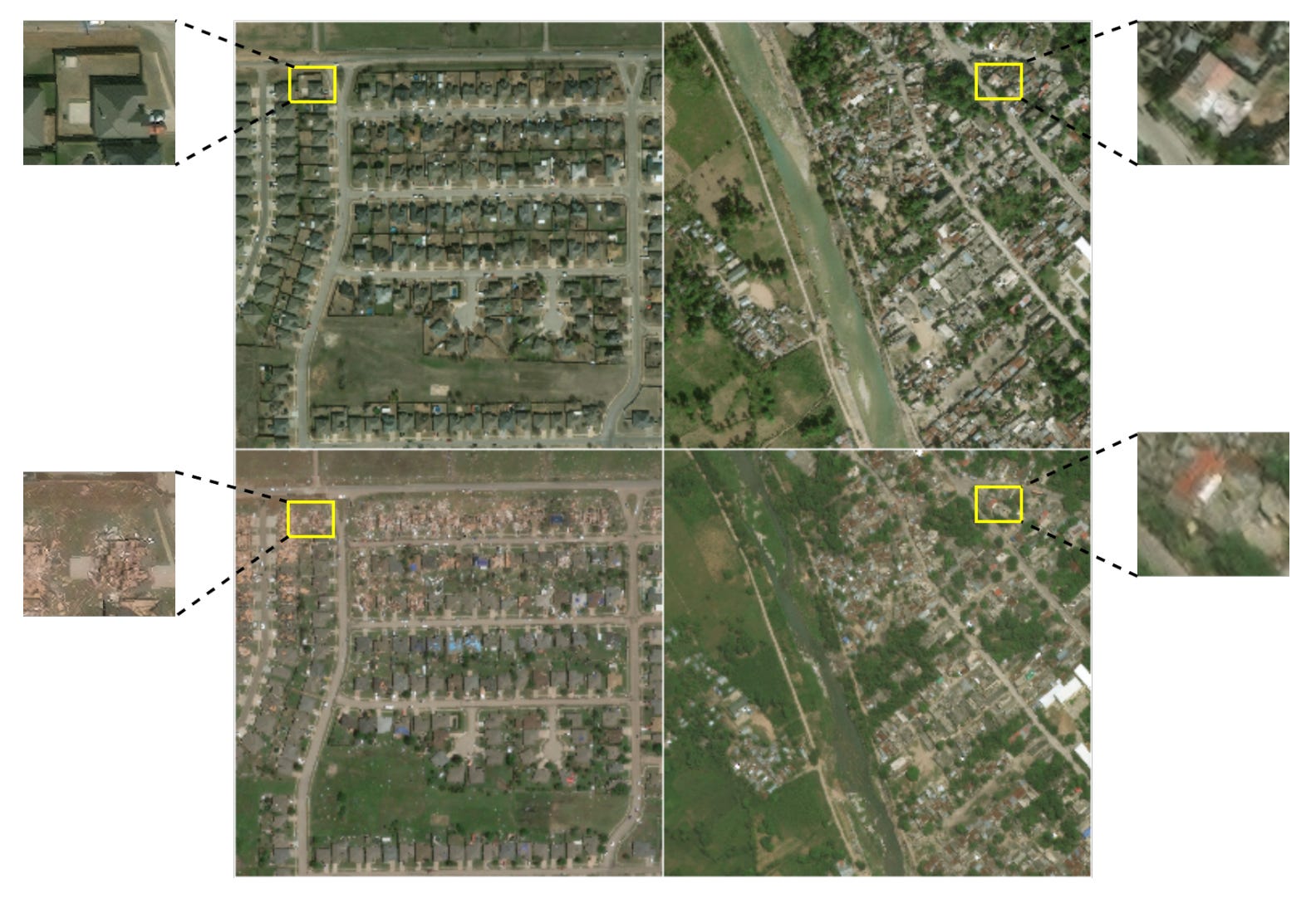
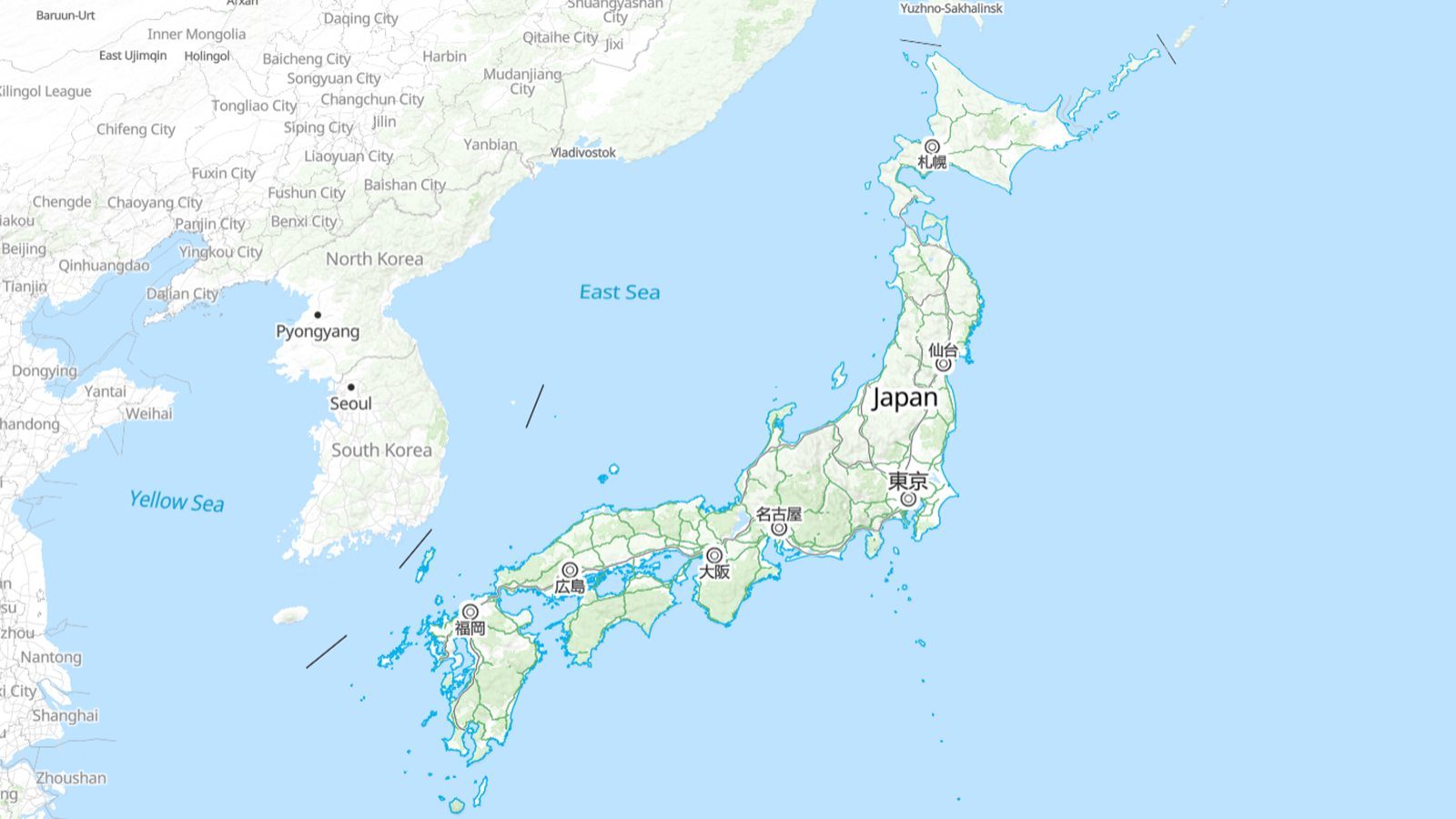


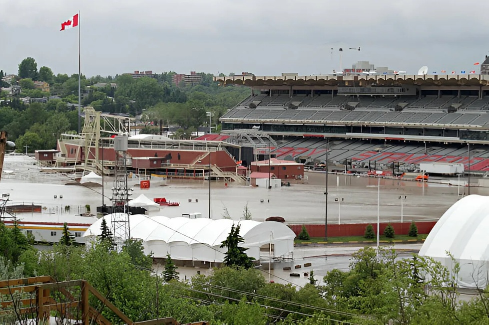
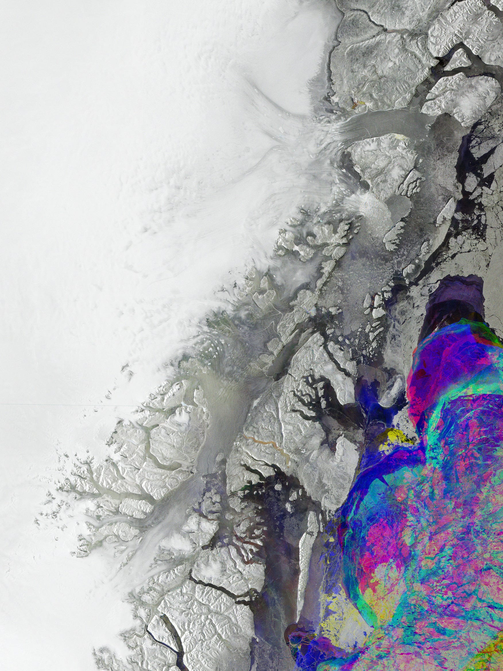

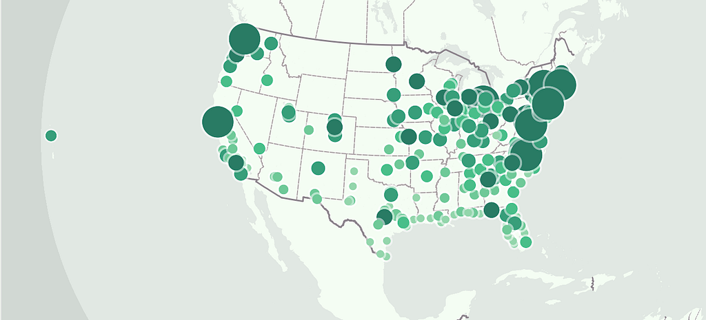

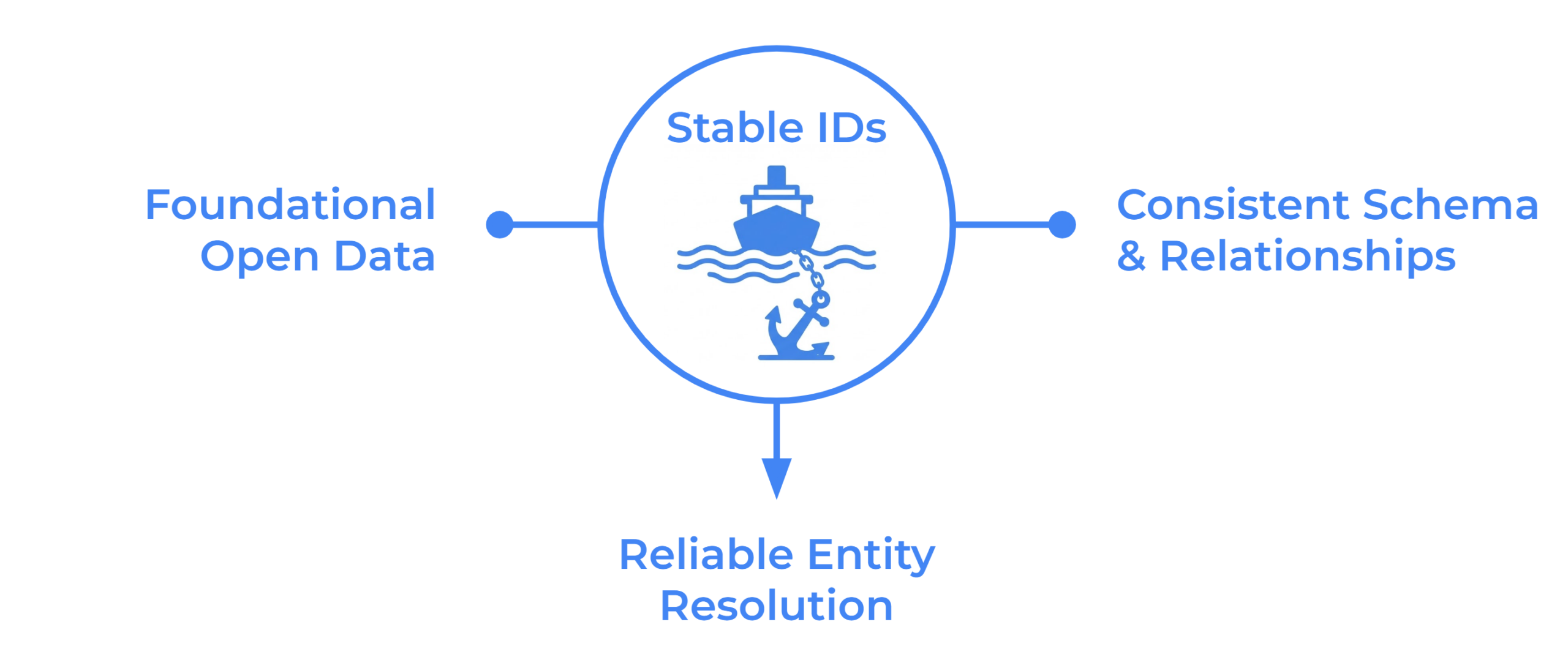
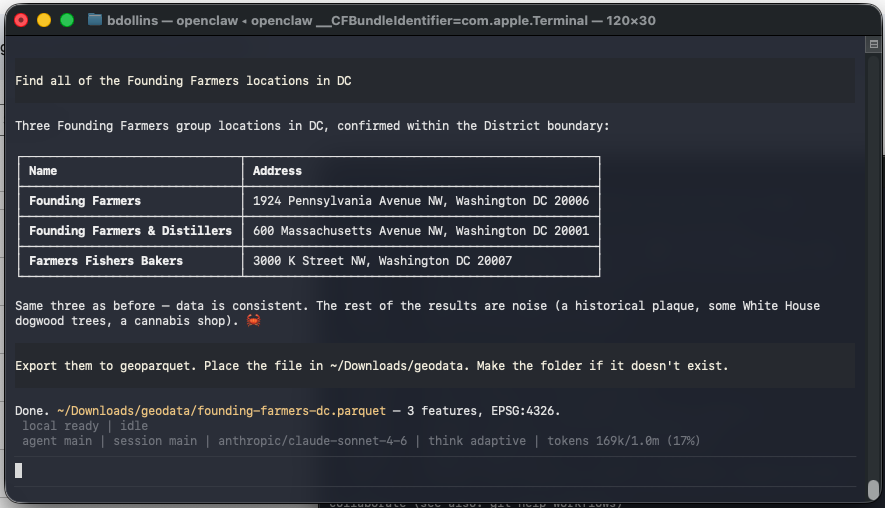


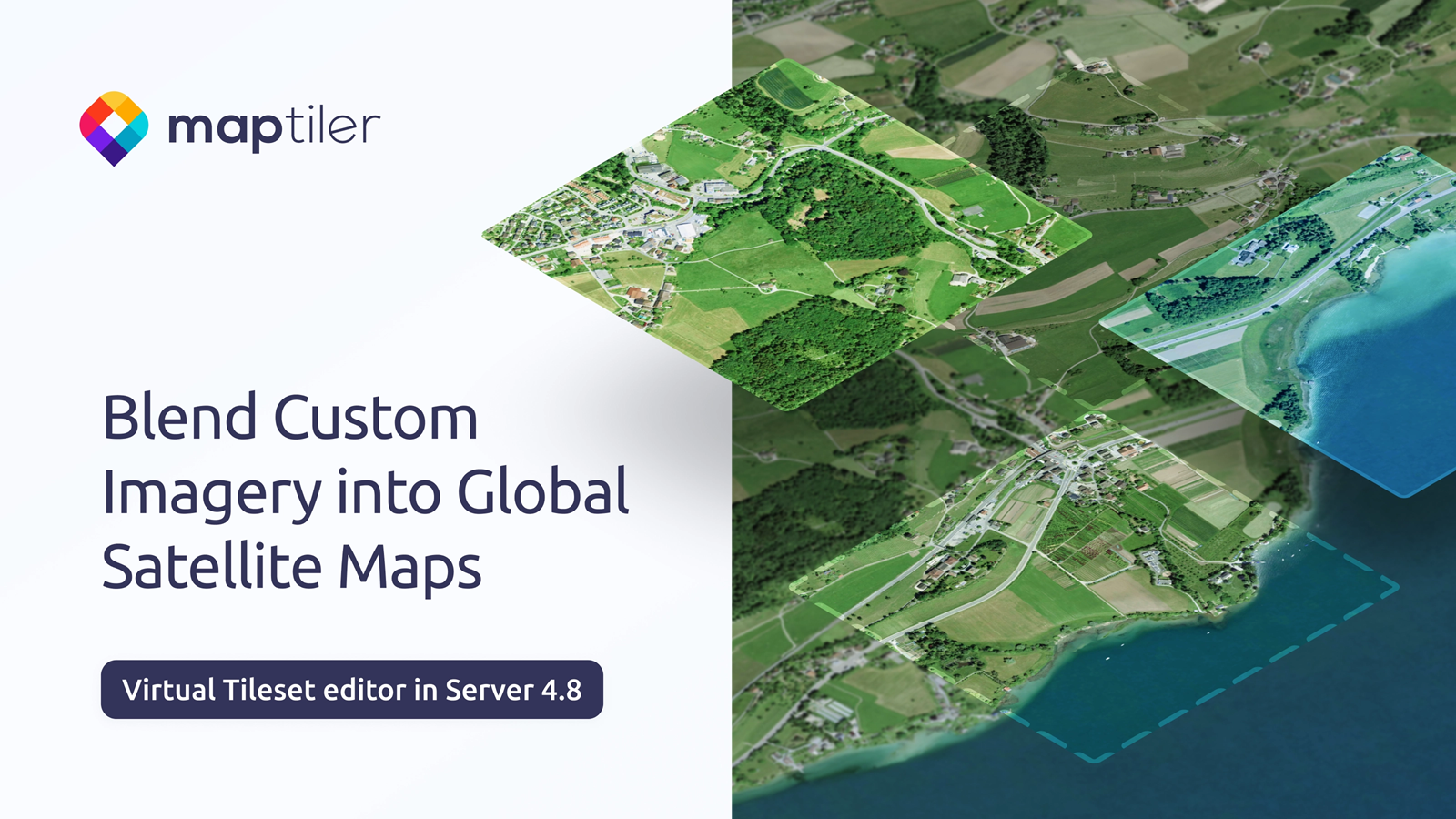


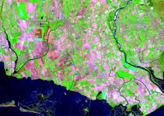
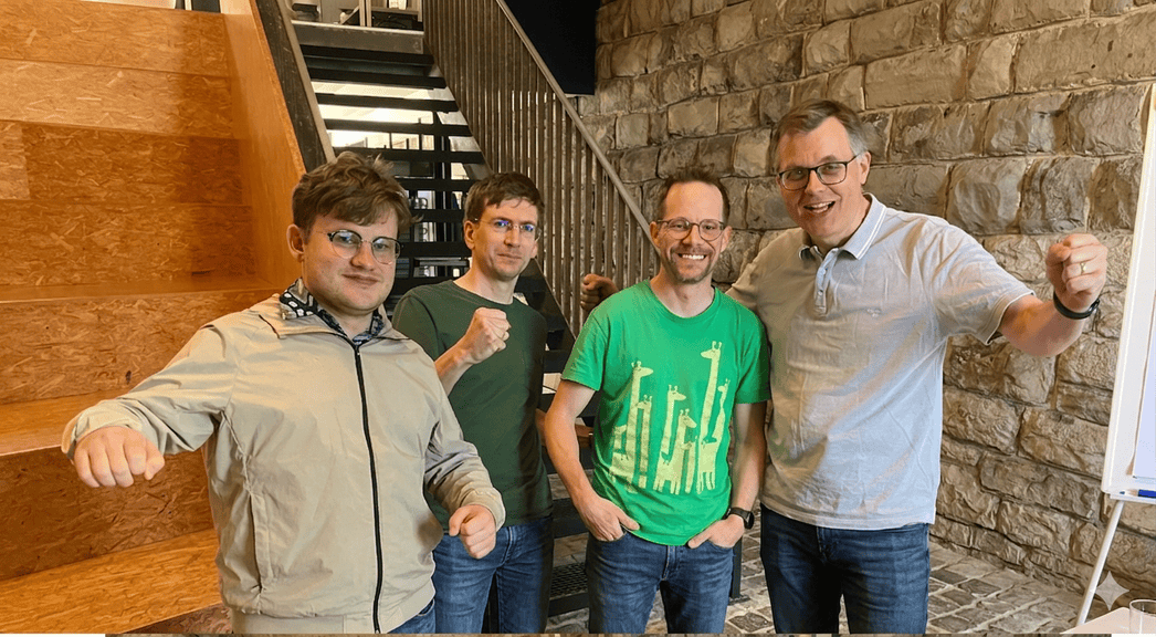
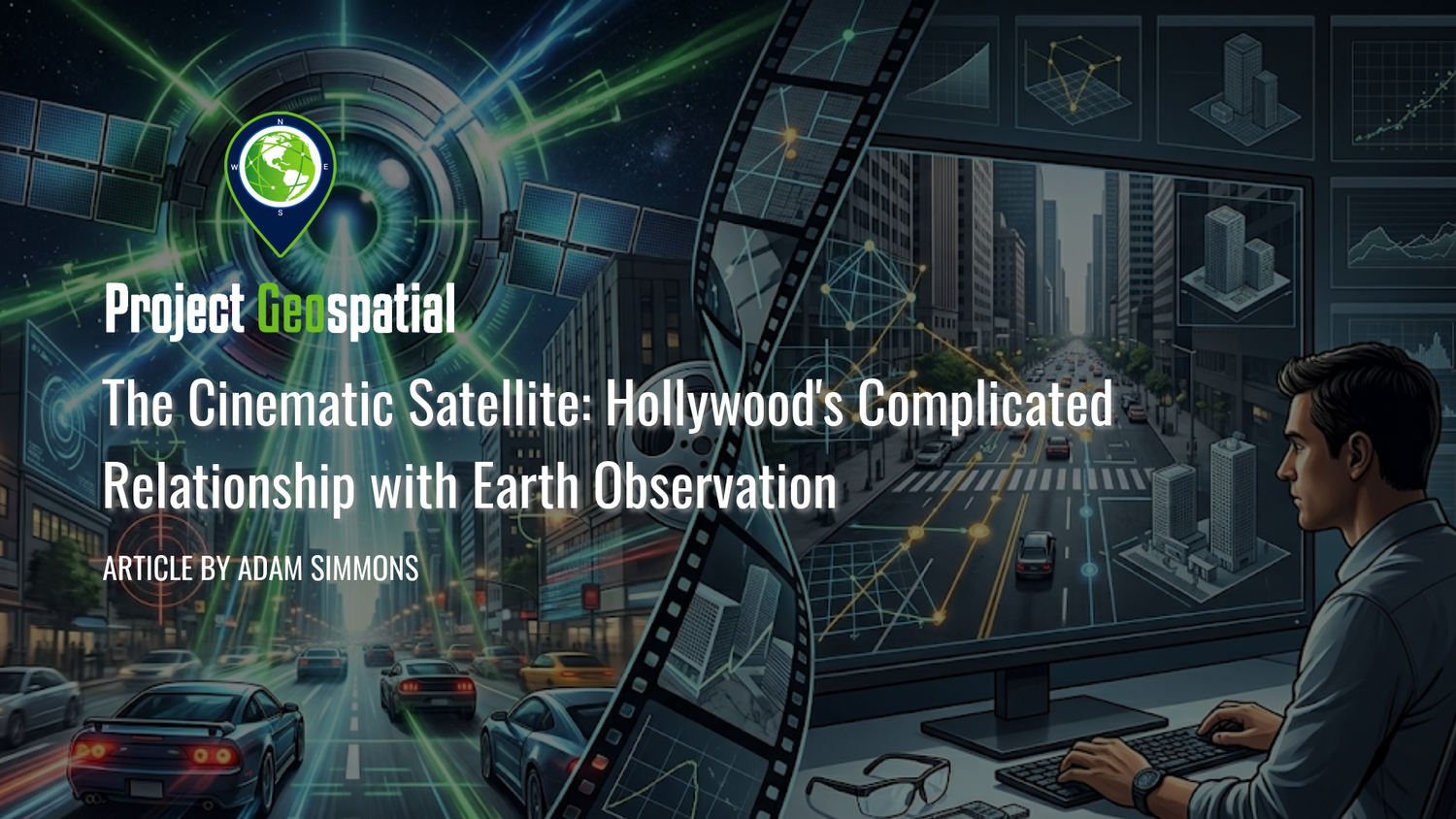
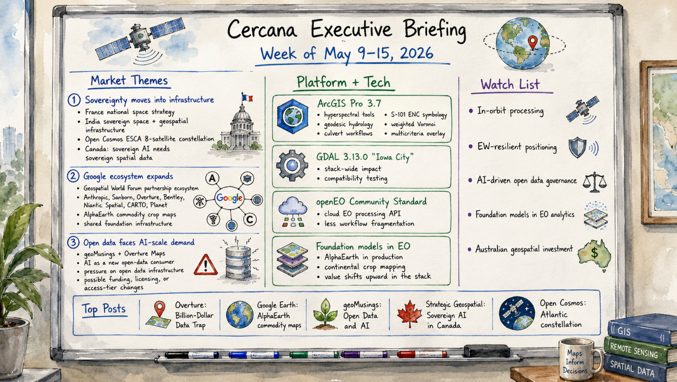


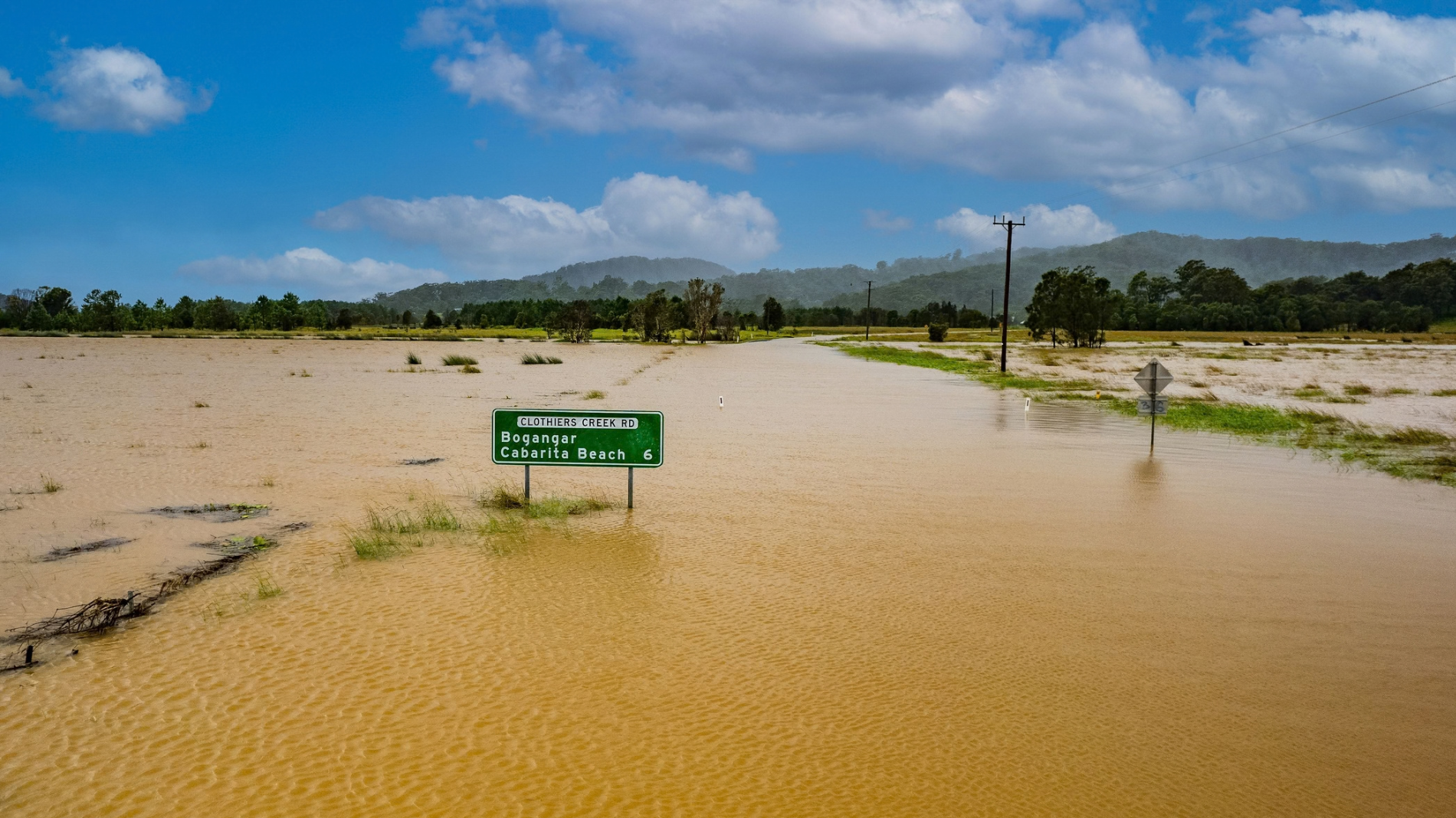

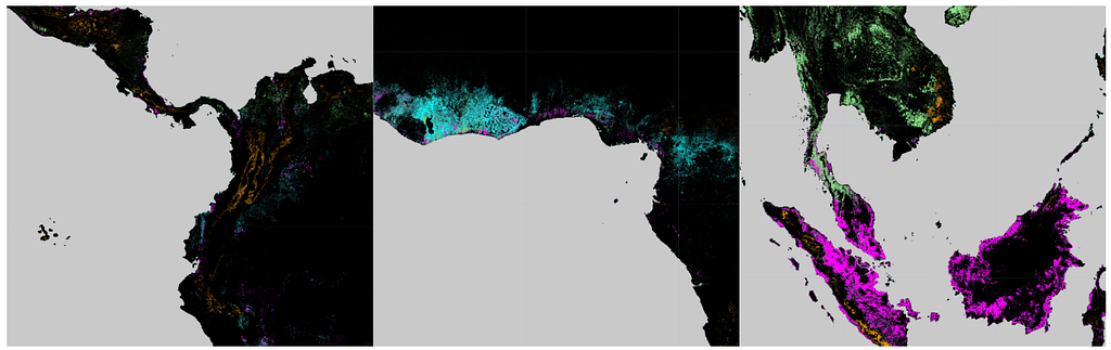

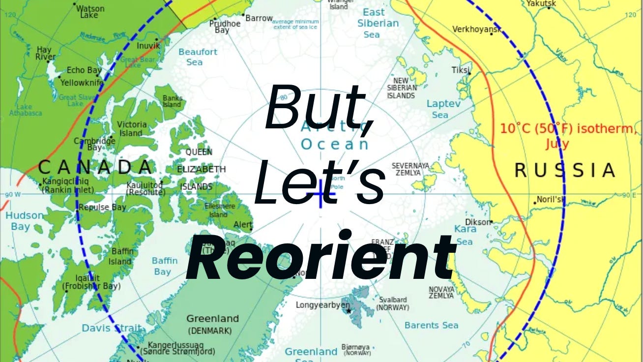
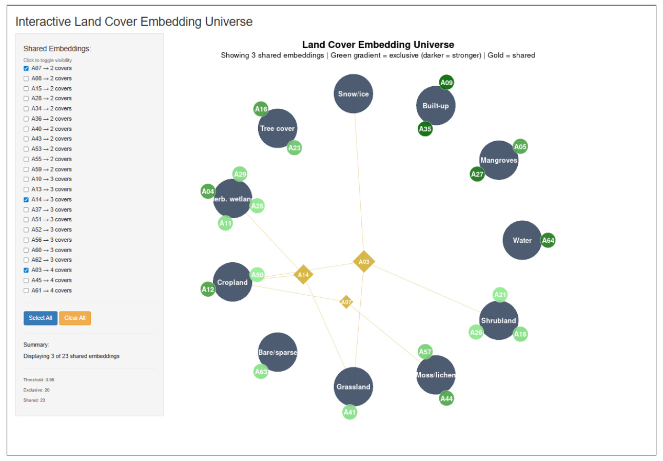
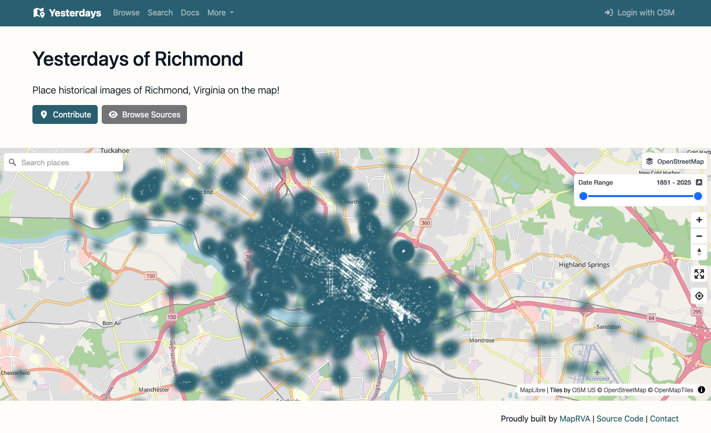


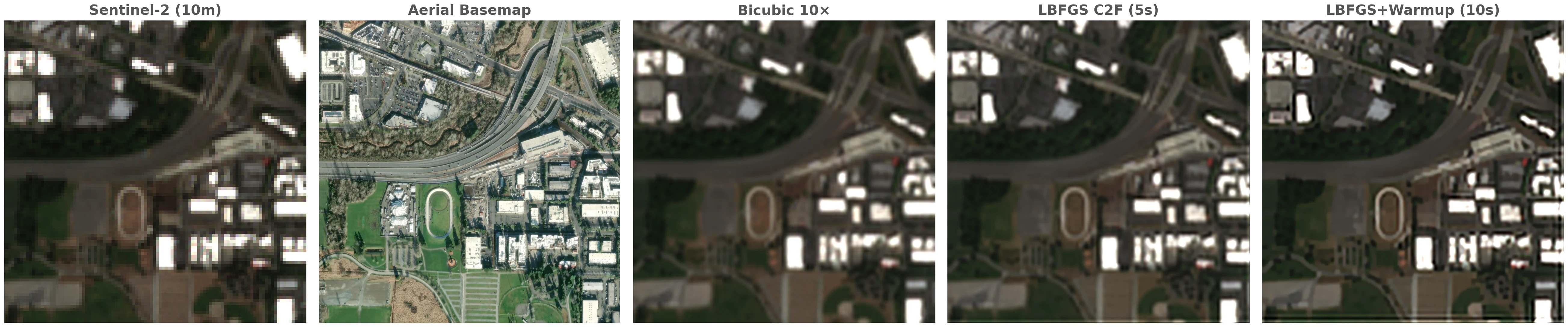


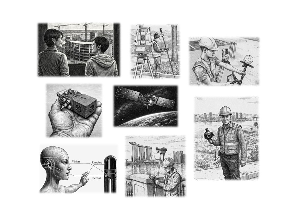


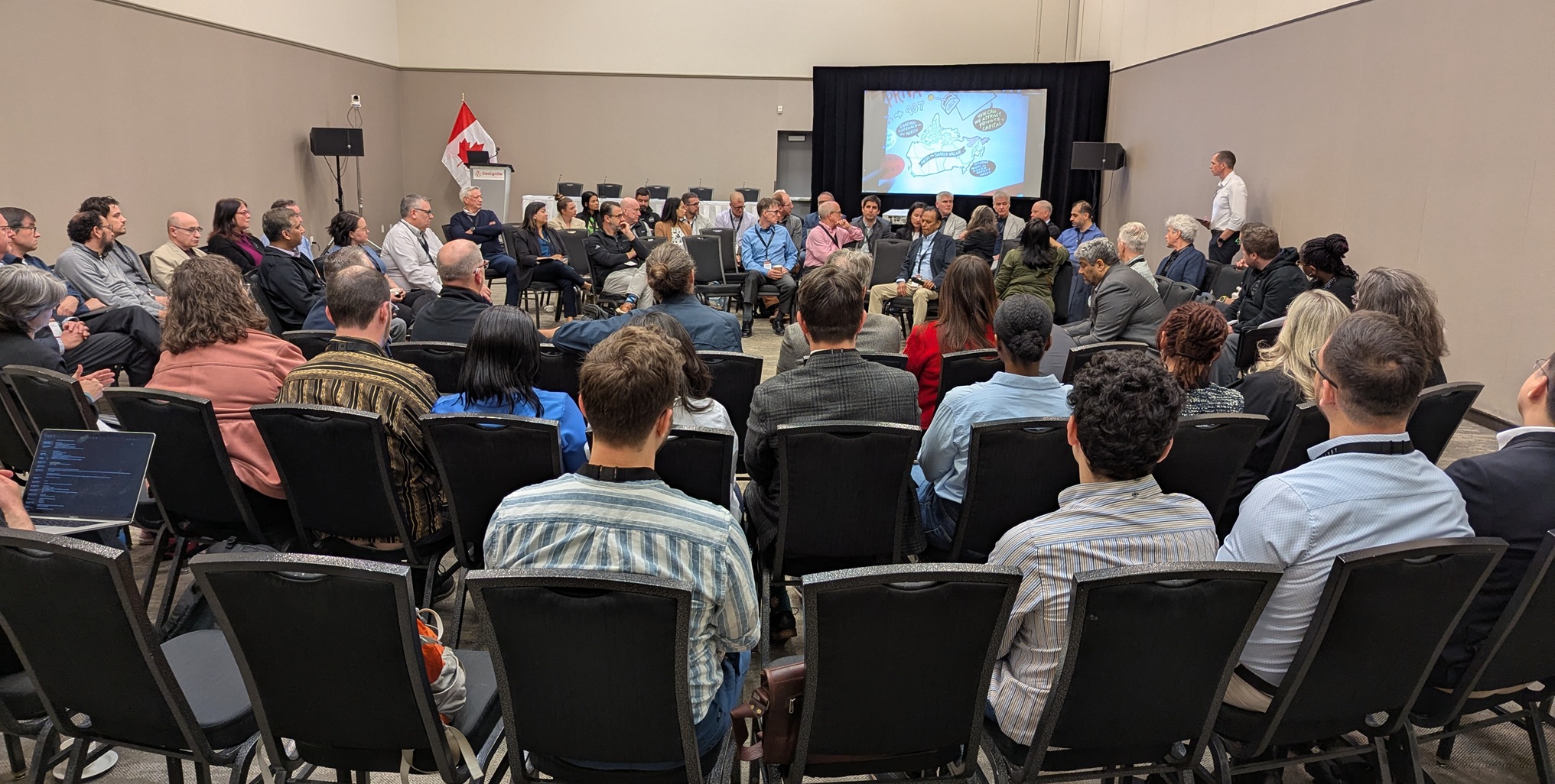


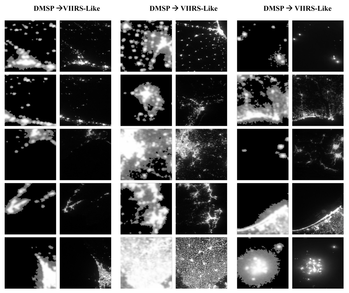

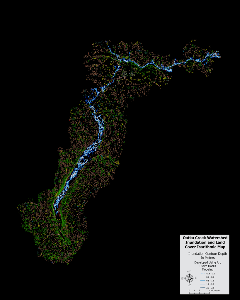

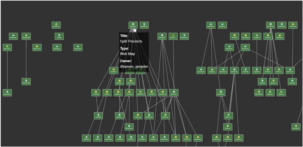
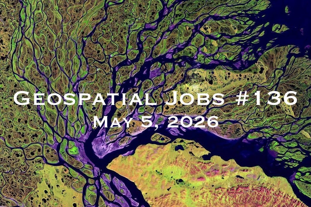


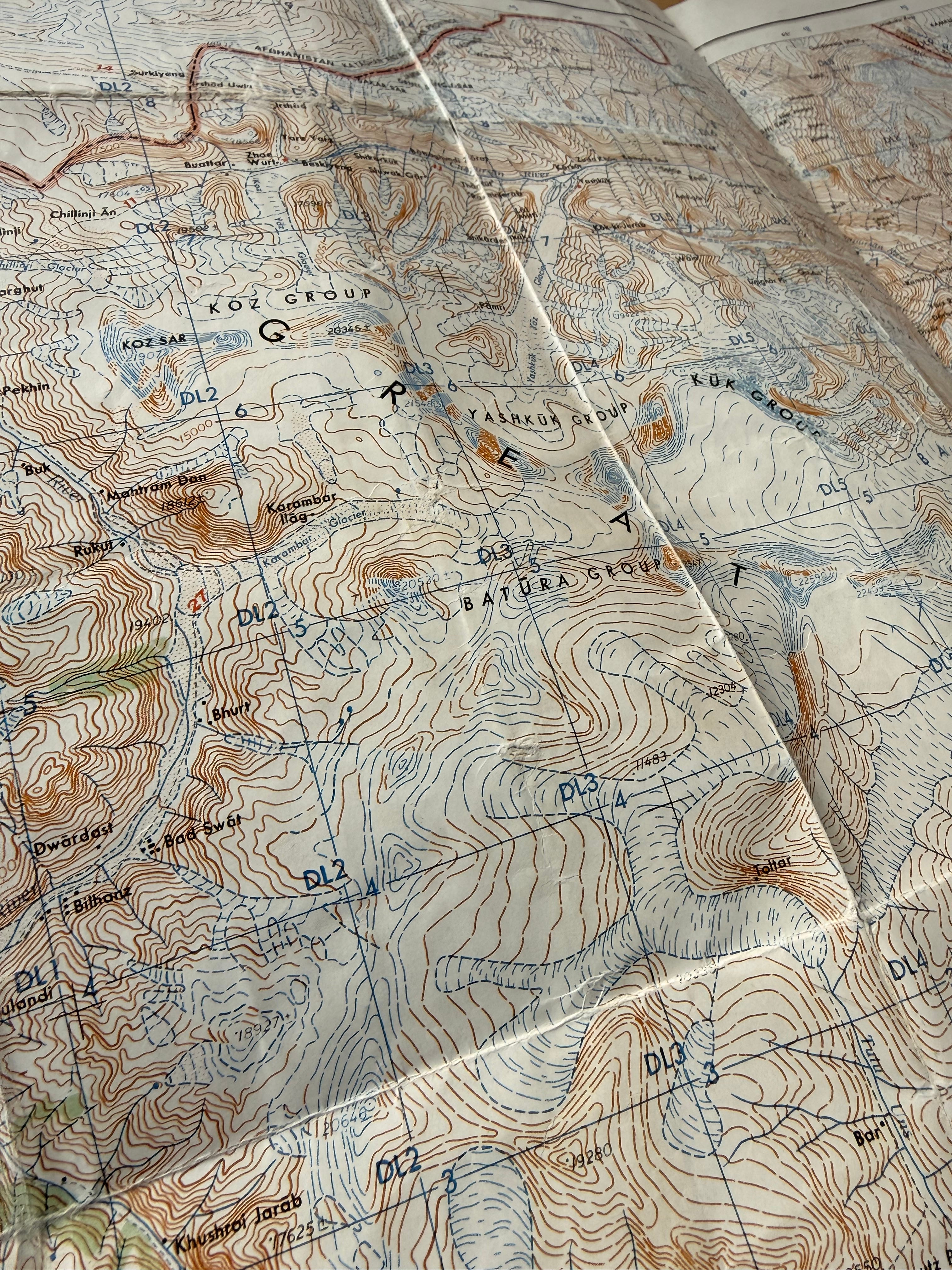


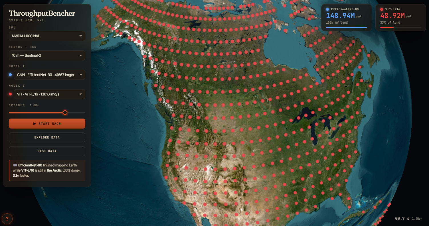

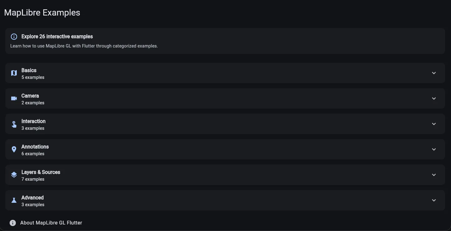


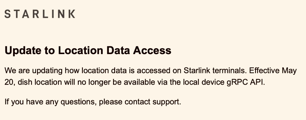
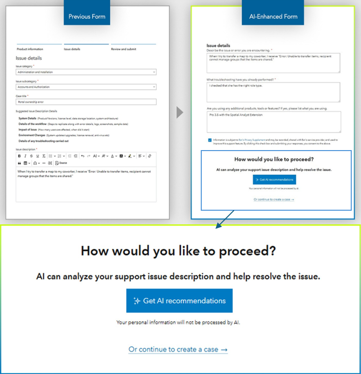


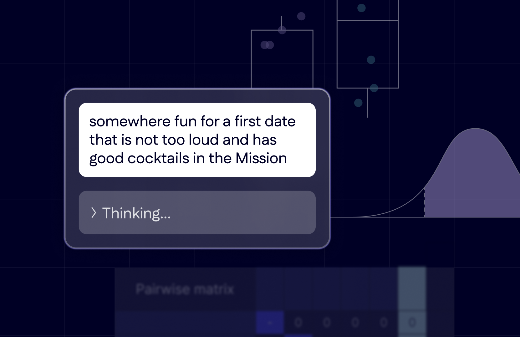
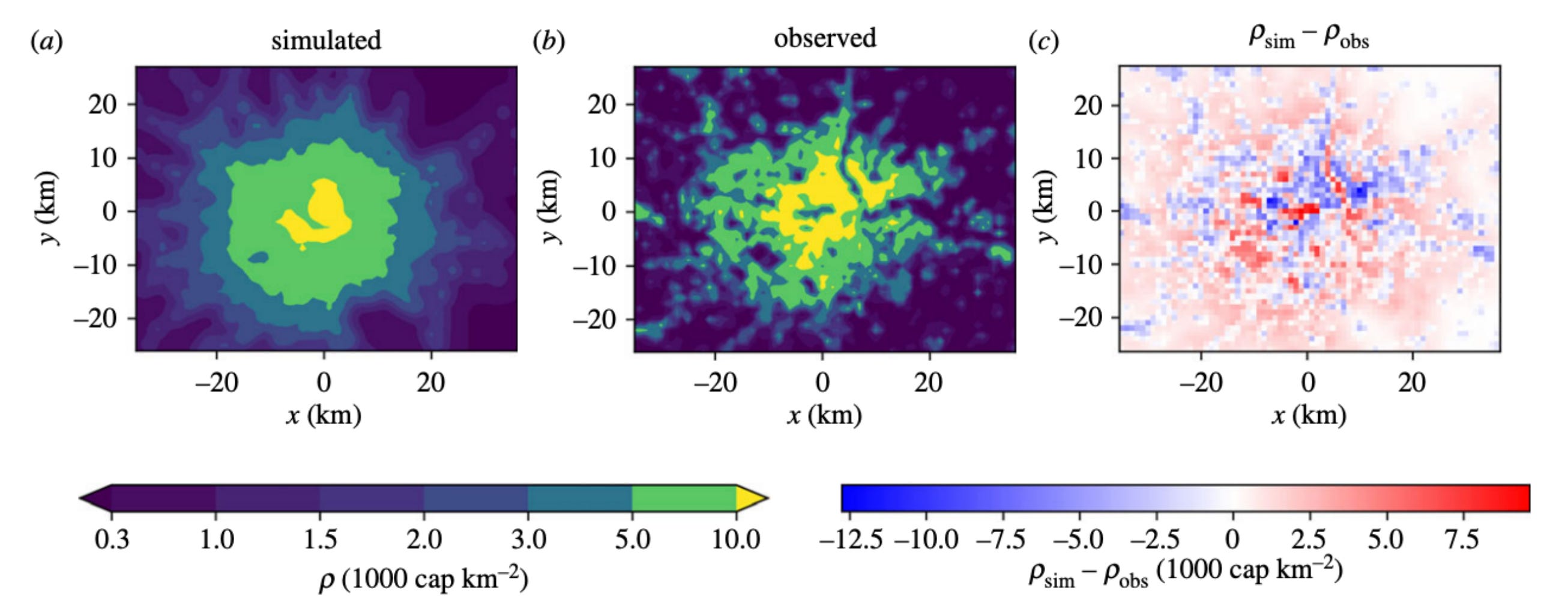


![Oslandia - (Fr) [Témoignage client] Fabrice Thevenon et Karine Lesage, chefs de projet SIG à la DSIN du Conseil Départemental de la Haute Garonne](https://oslandia.com/wp-content/uploads/2026/04/t%C3%A9moignage-CD-Haute-Garonne-oslandia-vok.png)


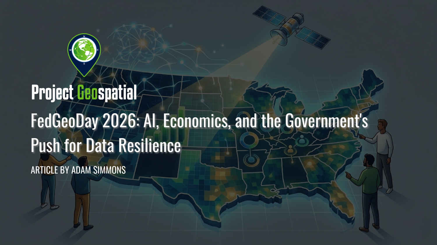
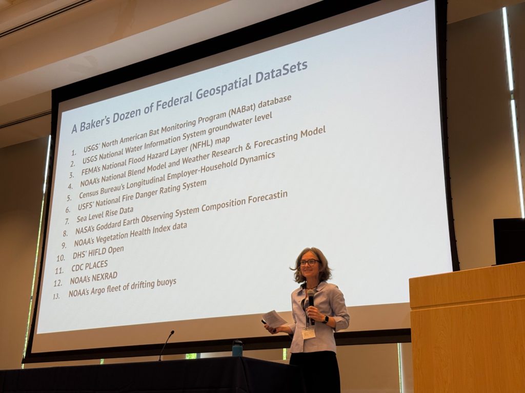


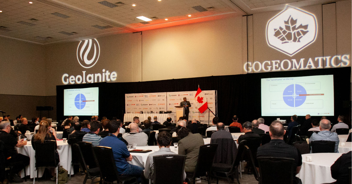
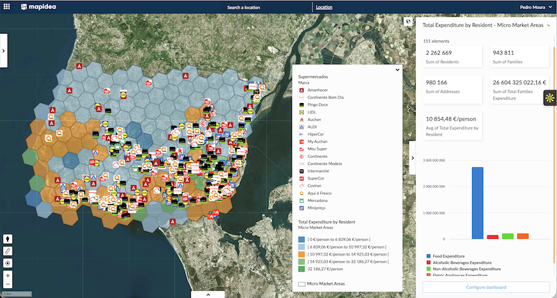
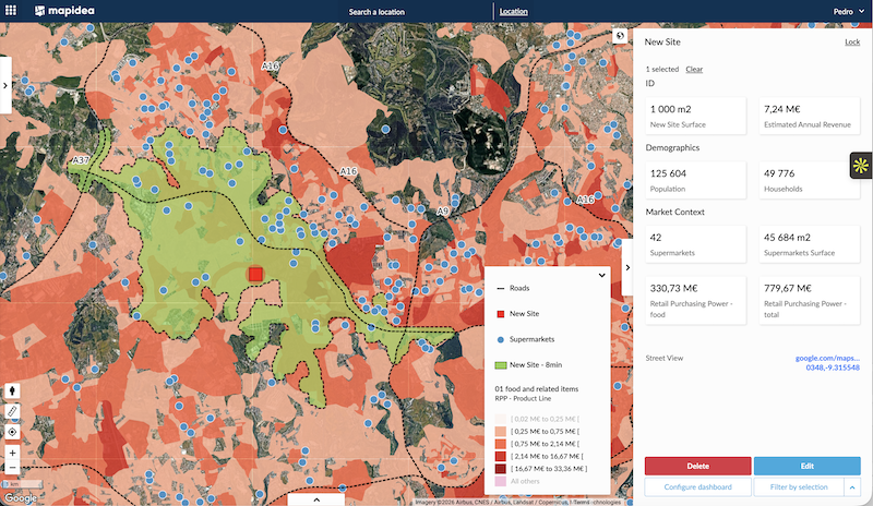
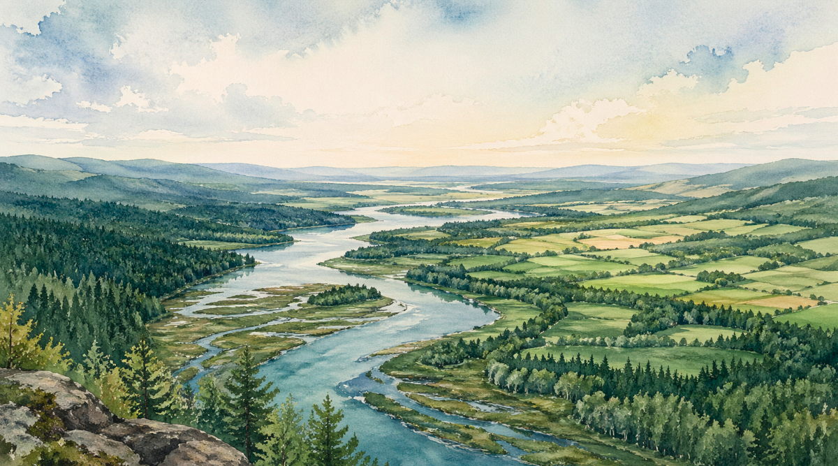

![Mergin Maps blog - [QGIS] From wishlist to app: Feature filtering is live](https://cdn.prod.website-files.com/64be358a4fb0e612b228bb9e/69eb362615bd3abfb19ecc28_Tak%20mapuj%20ne.jpg)

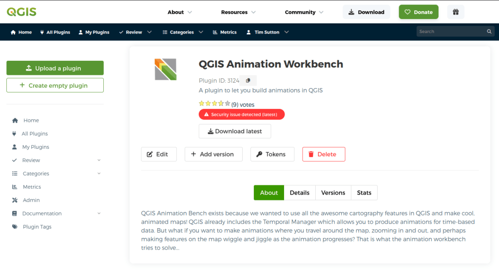


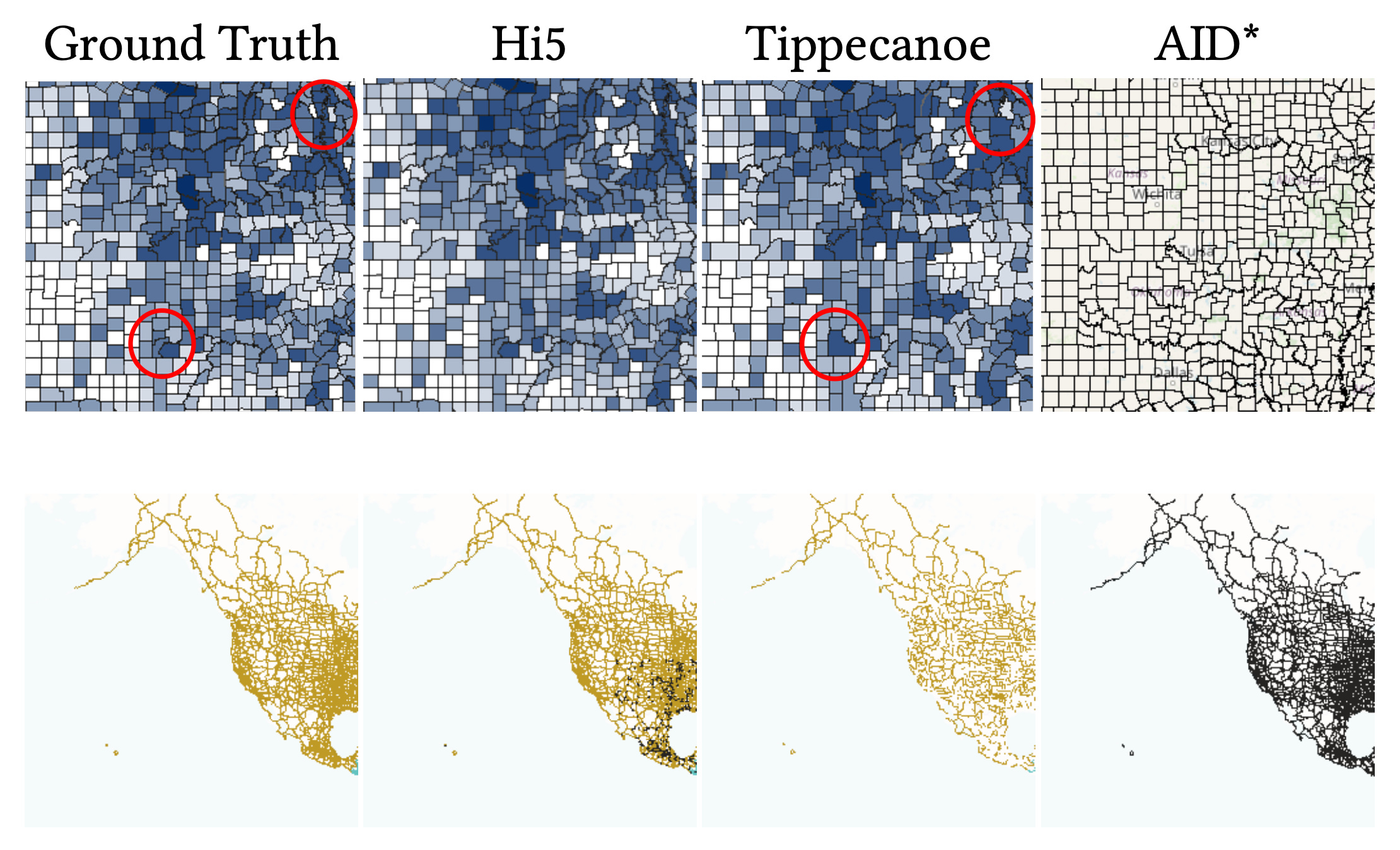


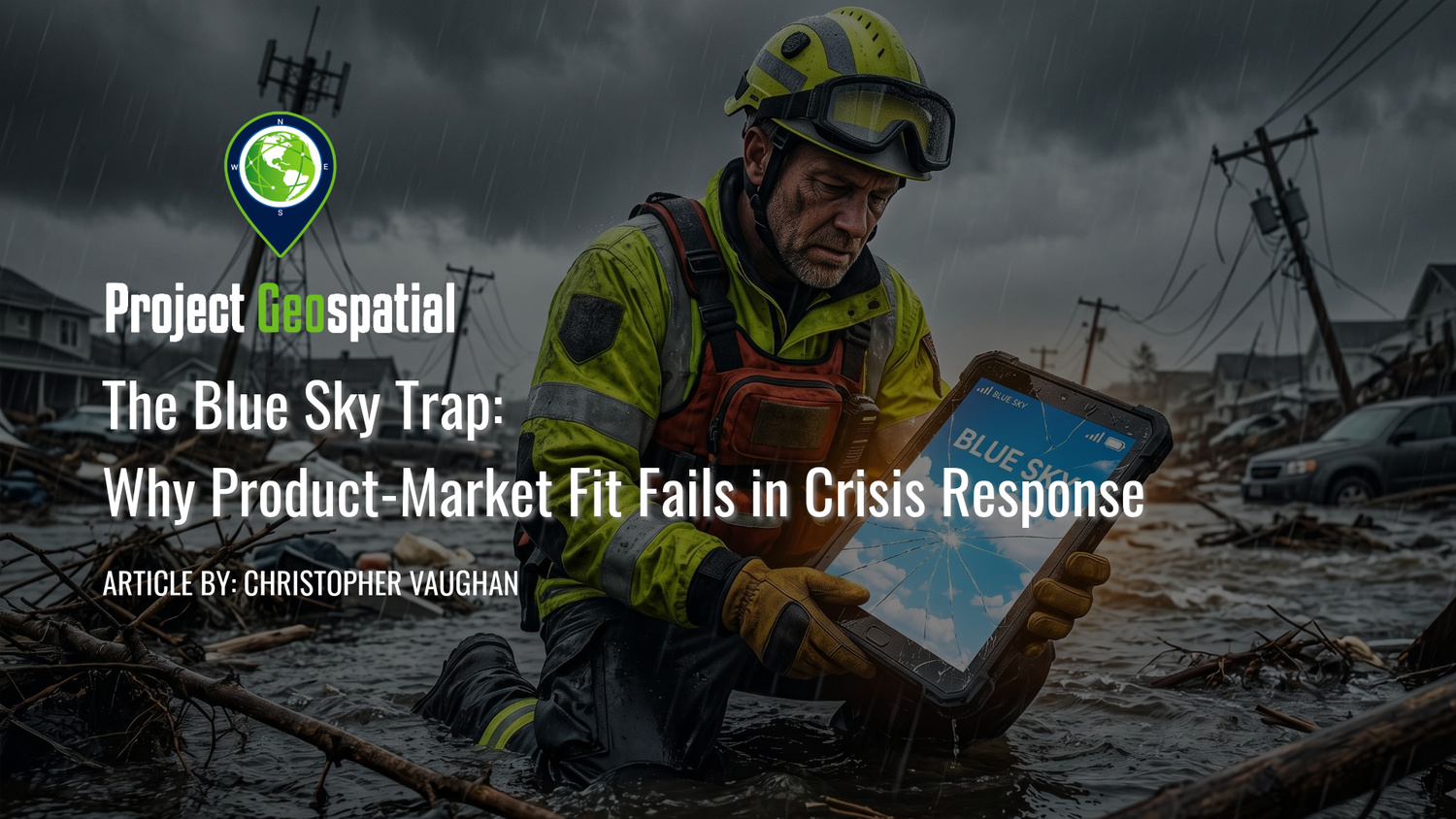


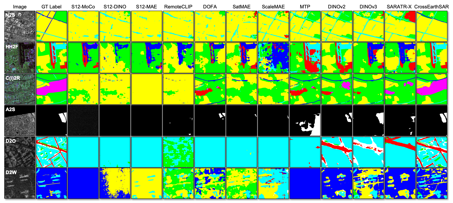


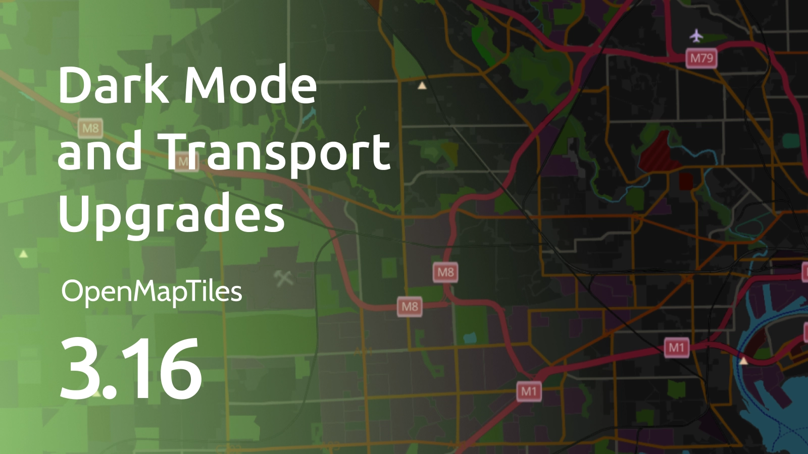

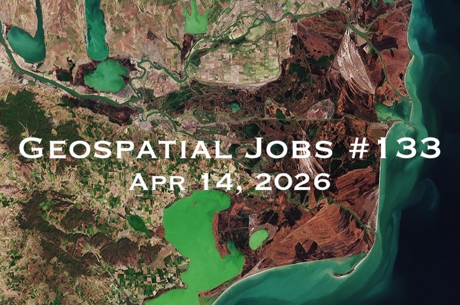
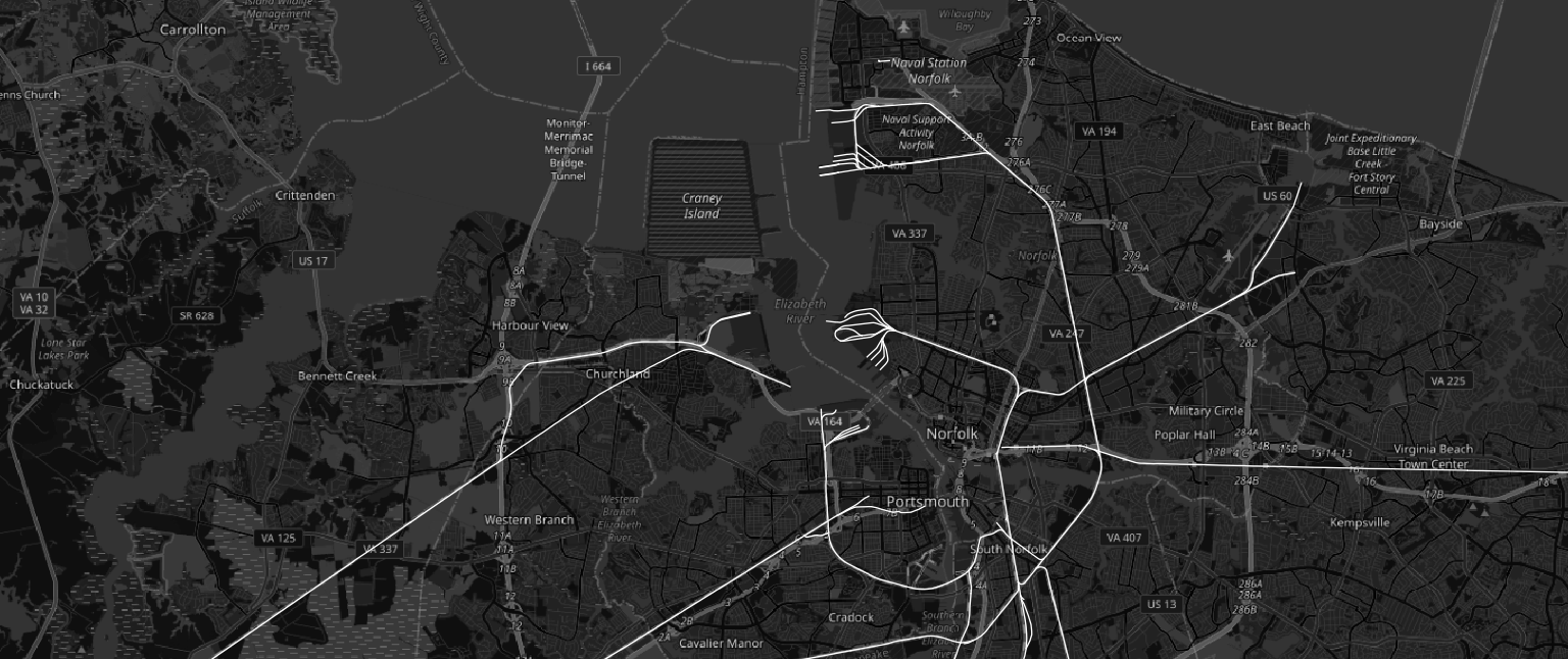


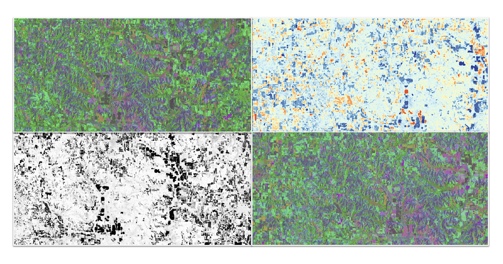

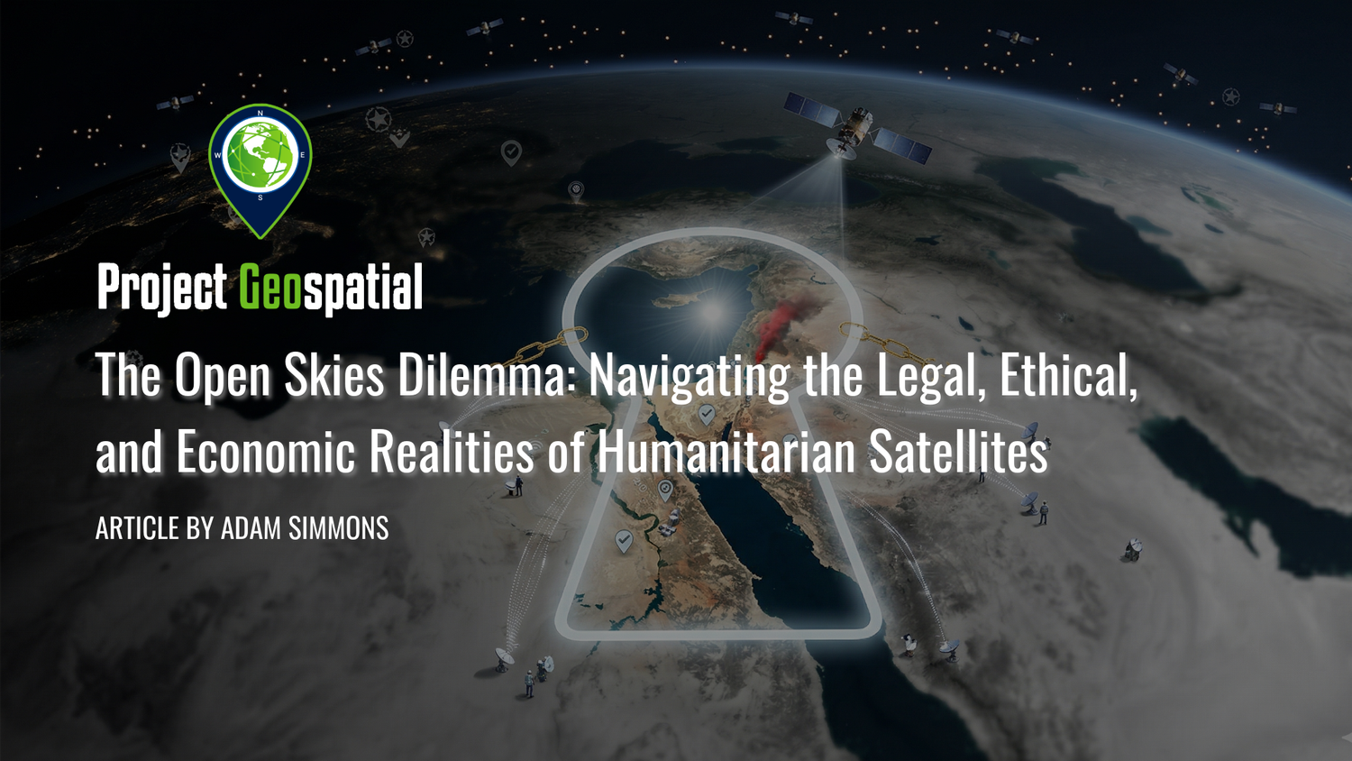


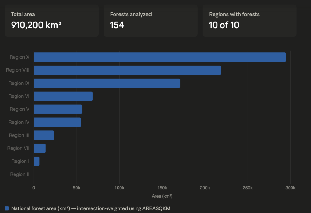
![Oslandia - (Fr) [Témoignage client] Julien Girard Claudon, DSI LPO AuRA](https://oslandia.com/wp-content/uploads/2026/03/t%C3%A9moignage-LPO-AuRA-oslandia.png)
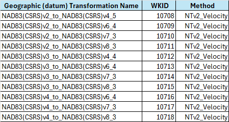

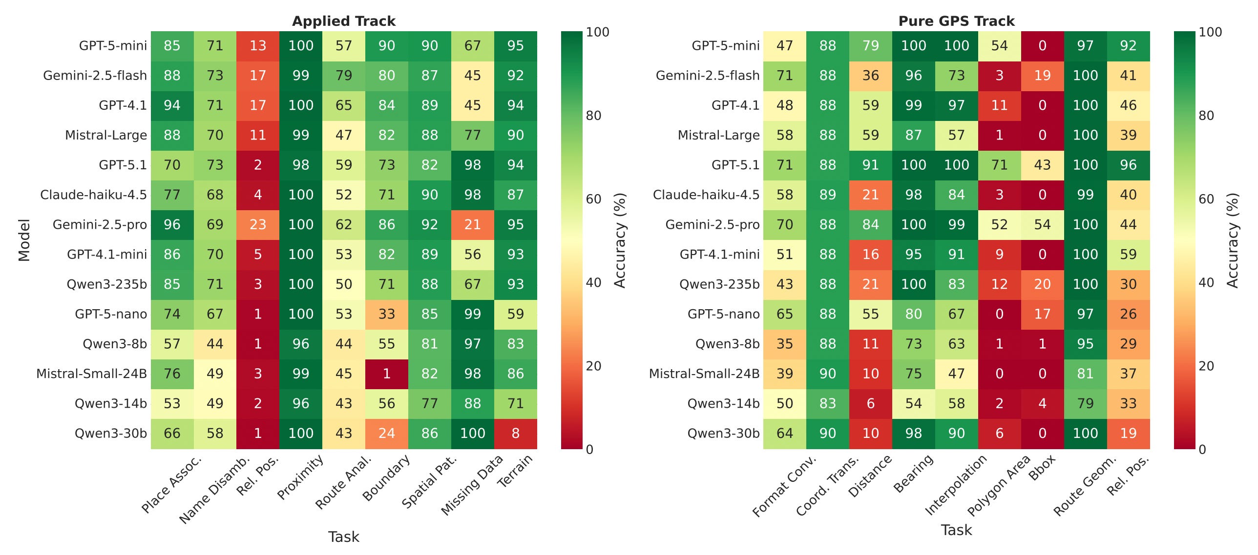
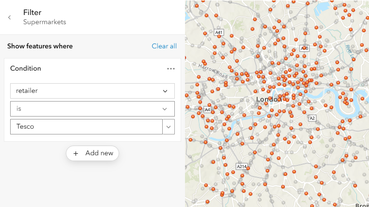
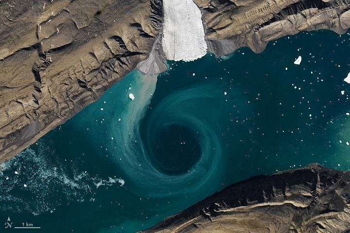
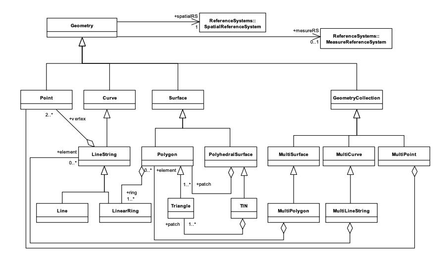


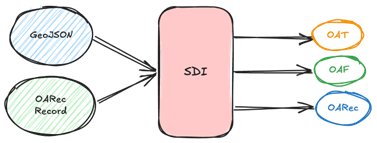

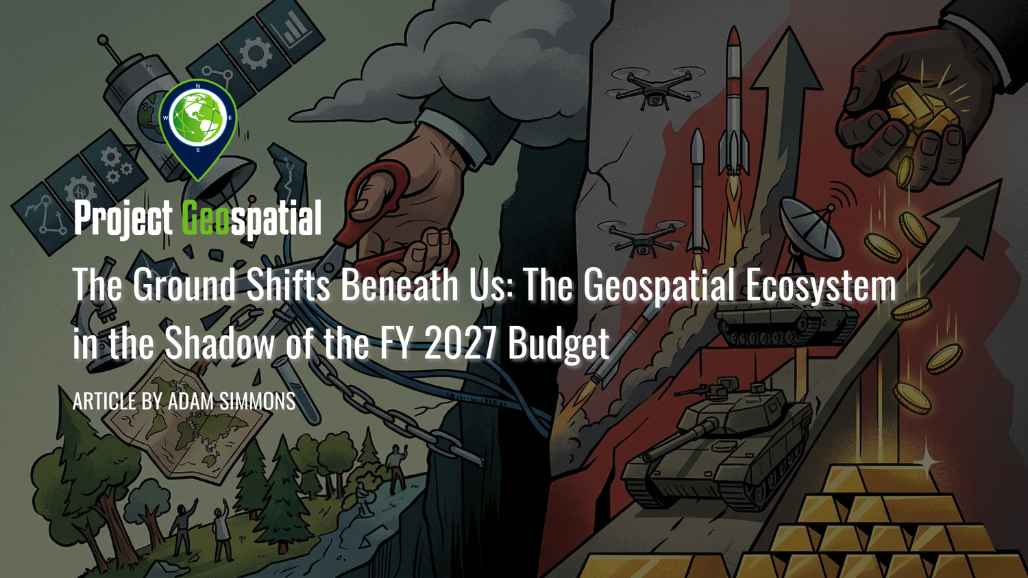

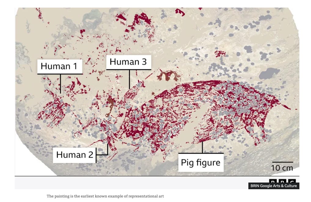


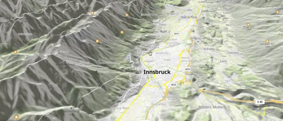


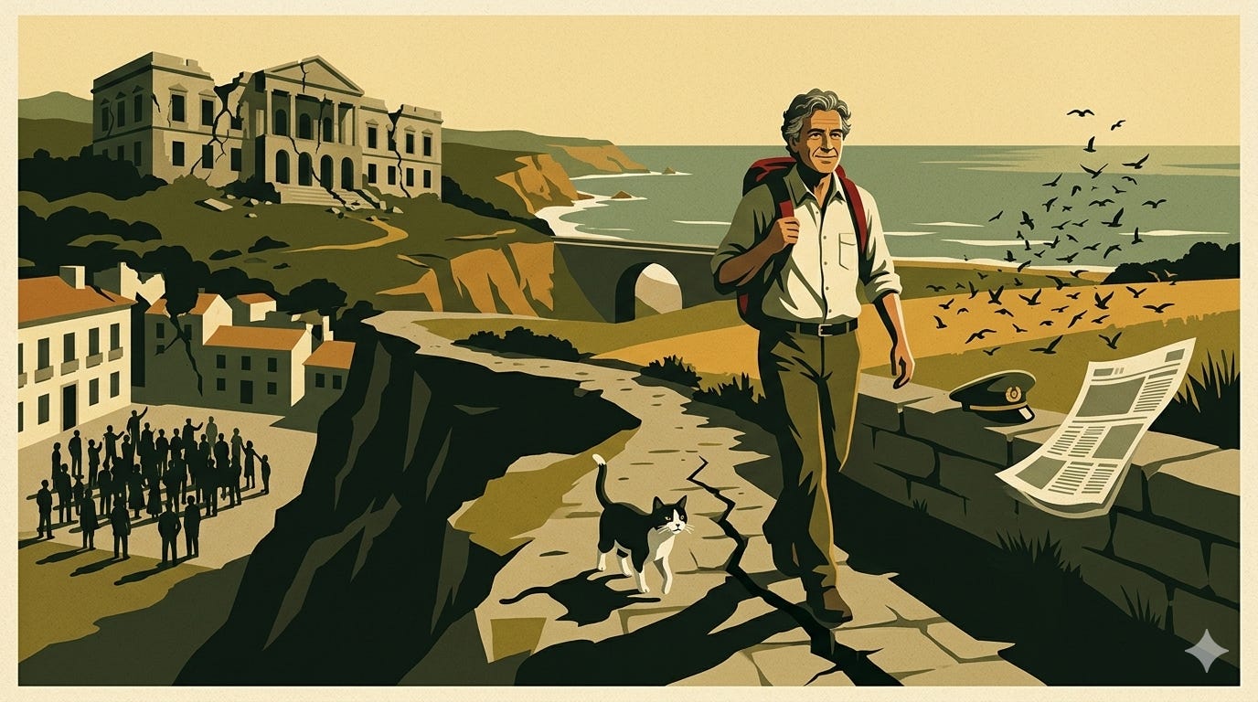


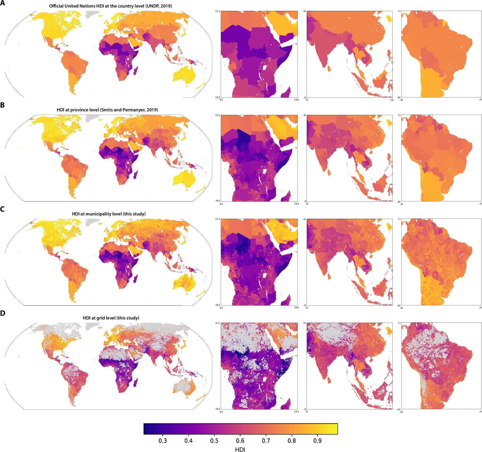

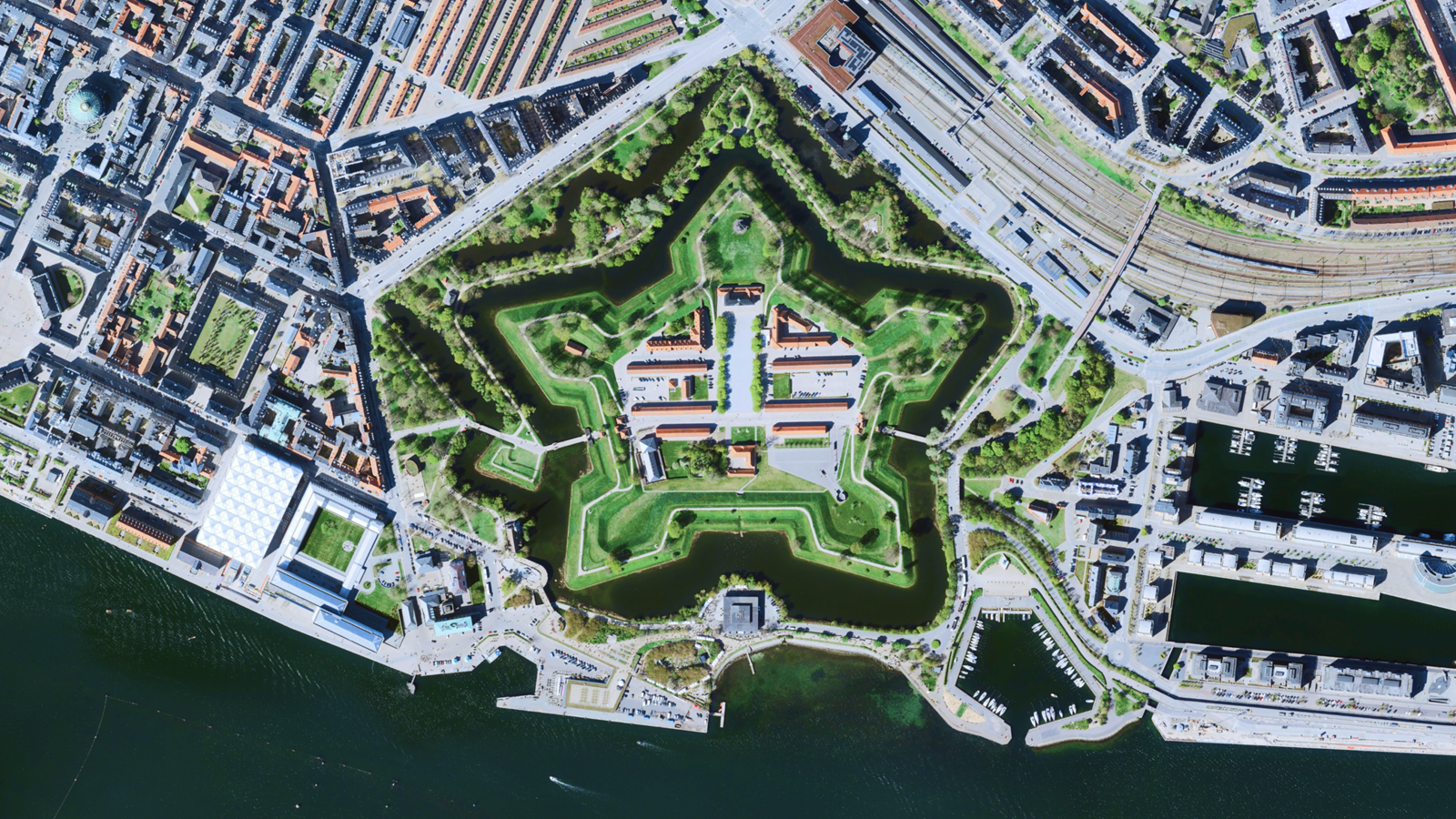


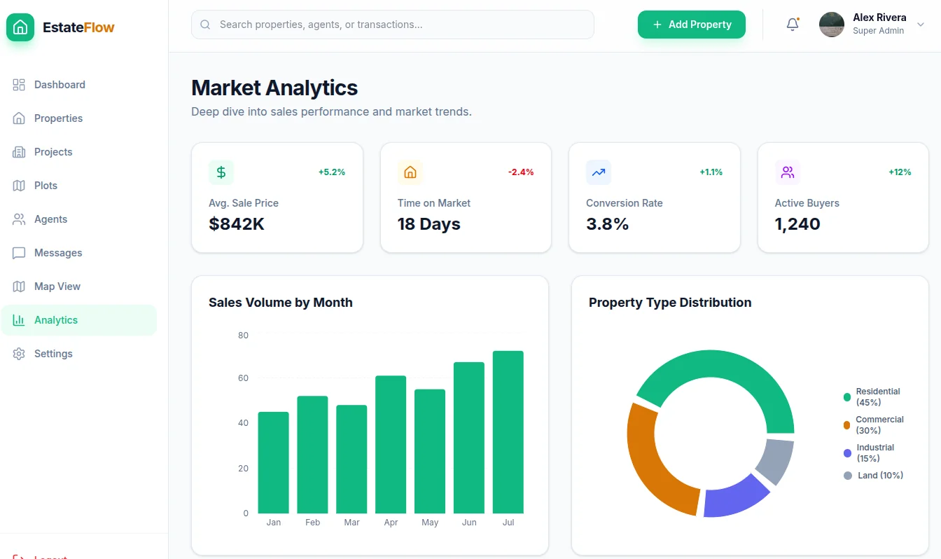


![Mergin Maps blog - [QGIS] Support tip - using conditions to improve your Mergin Maps survey](https://cdn.prod.website-files.com/64be358a4fb0e612b228bb9e/69c4116715093bc84ca66407_Tak%20mapuj%20ne.jpg)

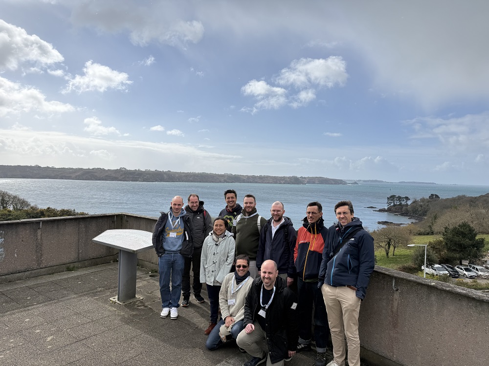
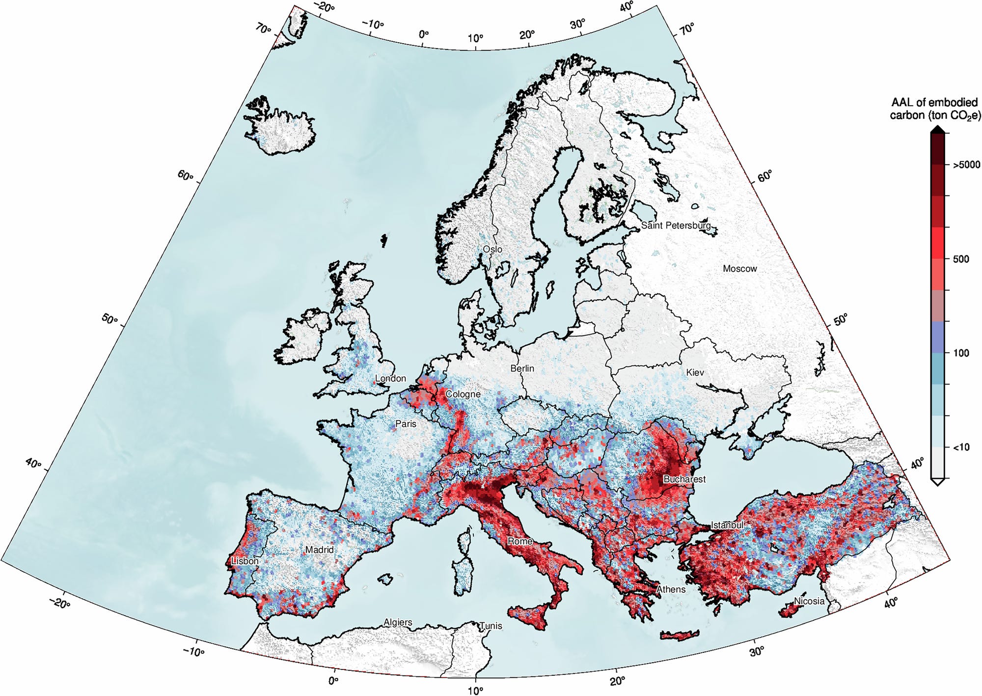

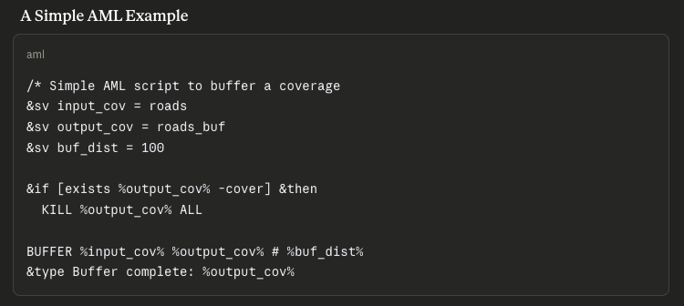

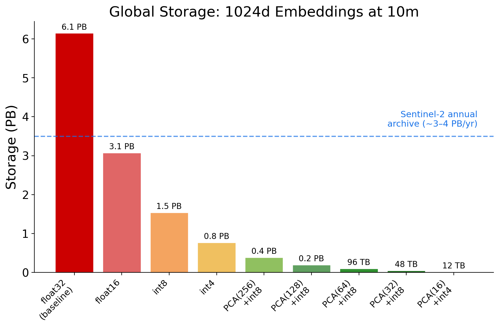


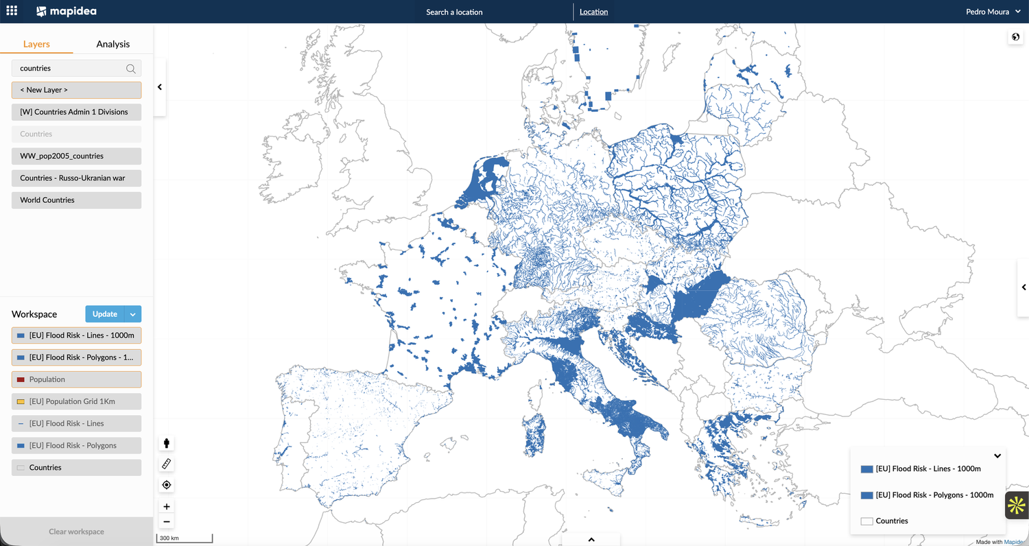
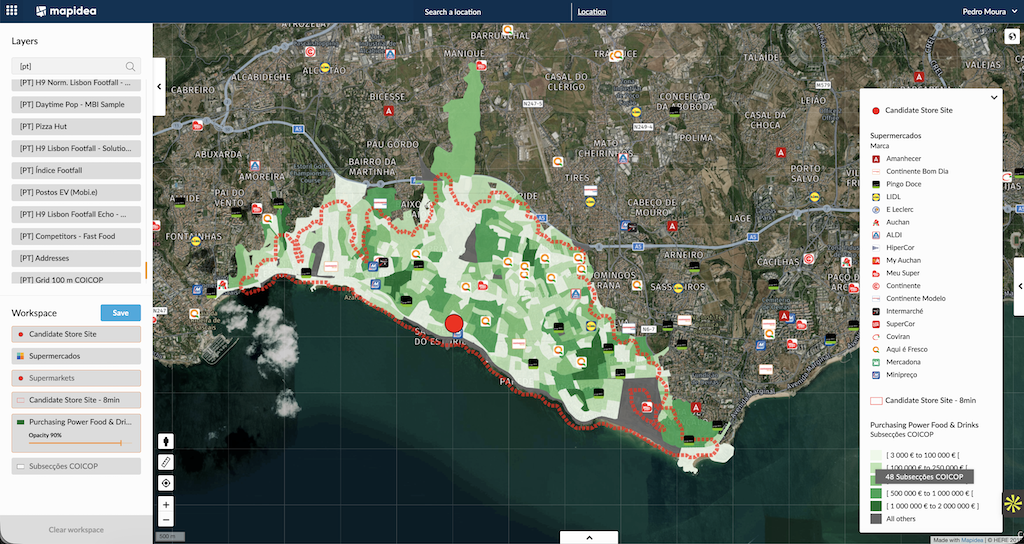


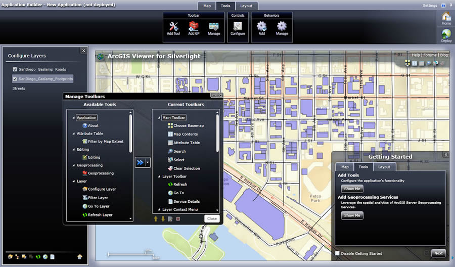
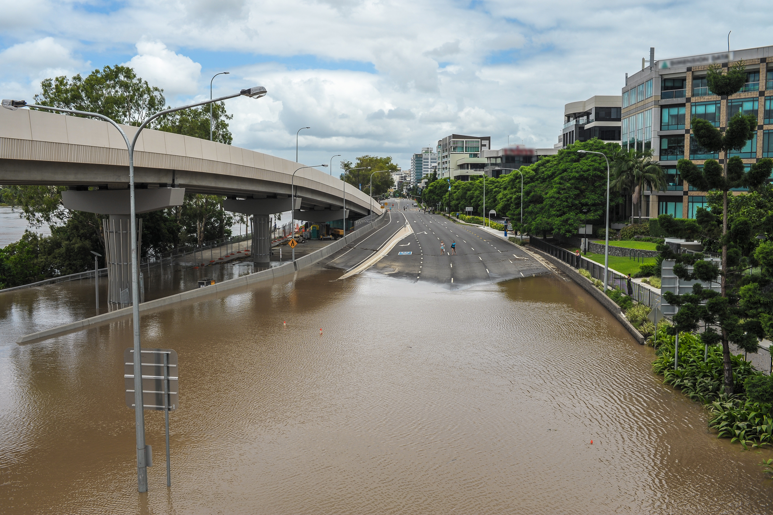


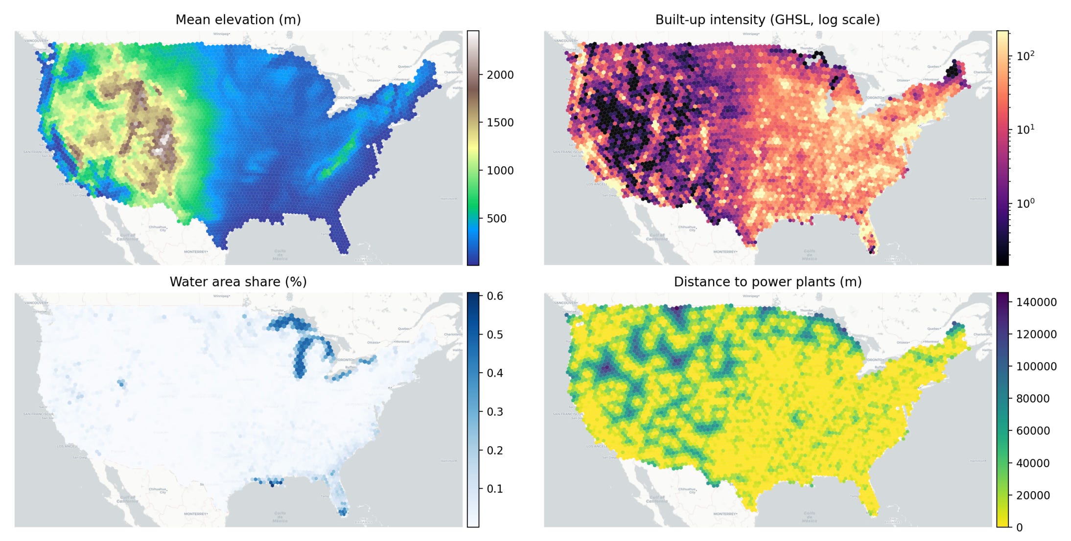
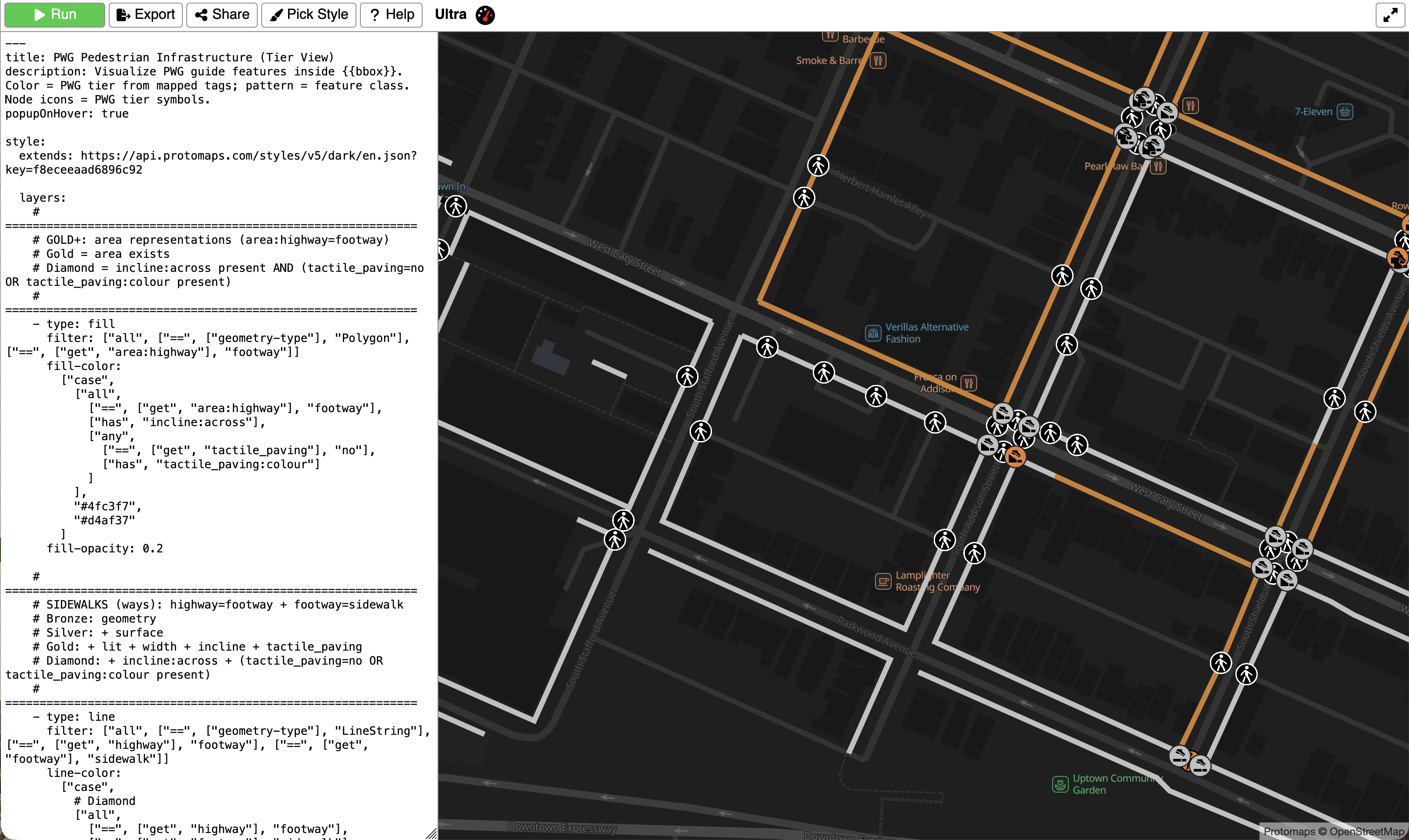

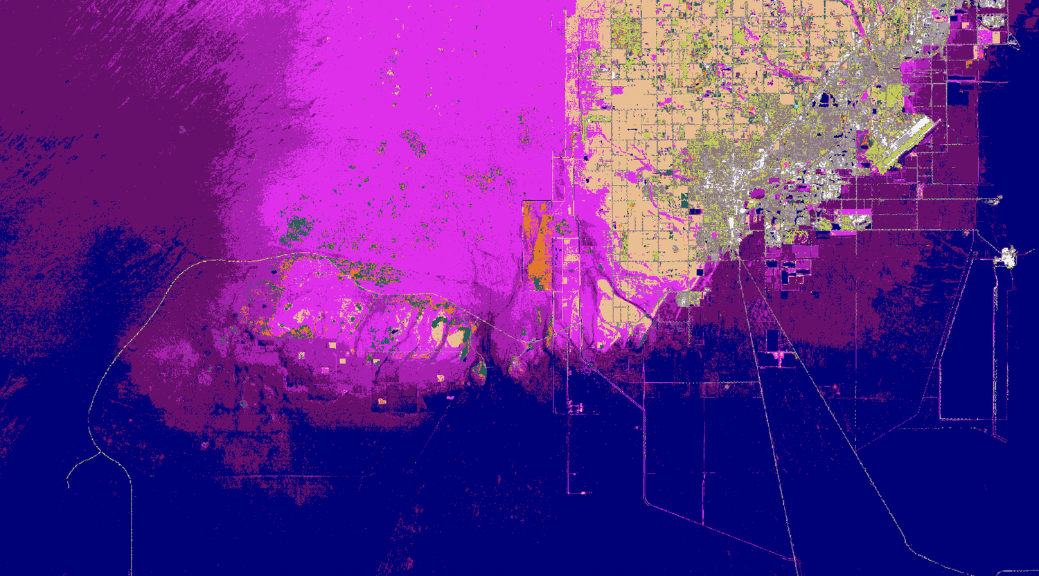

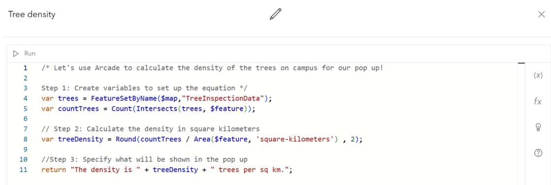
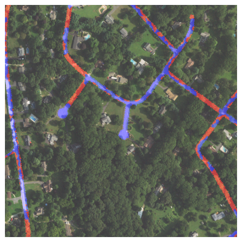


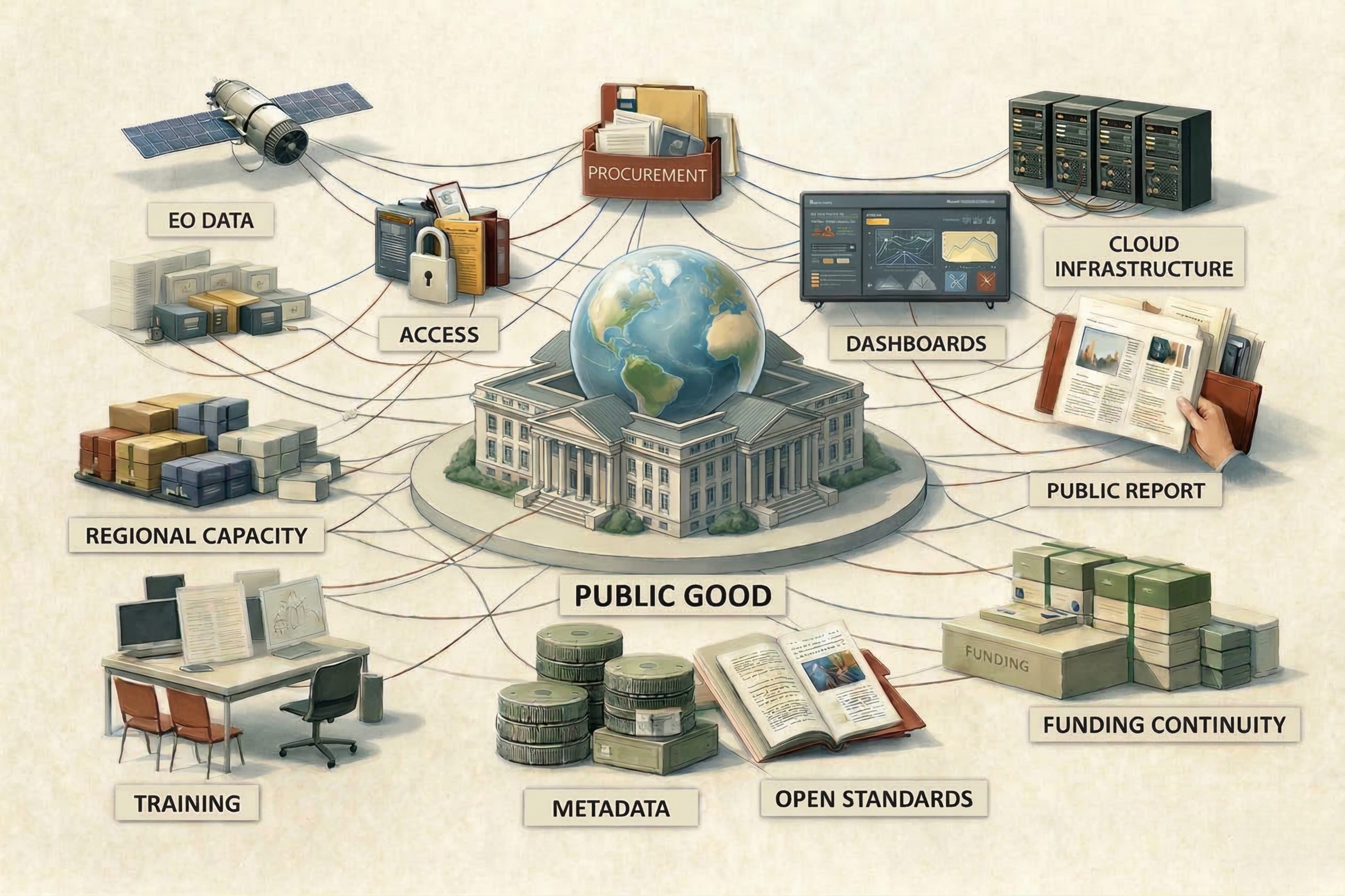


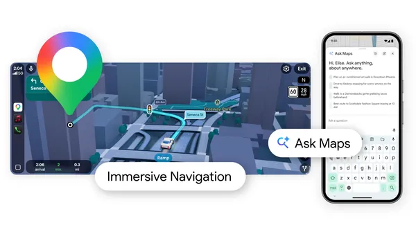

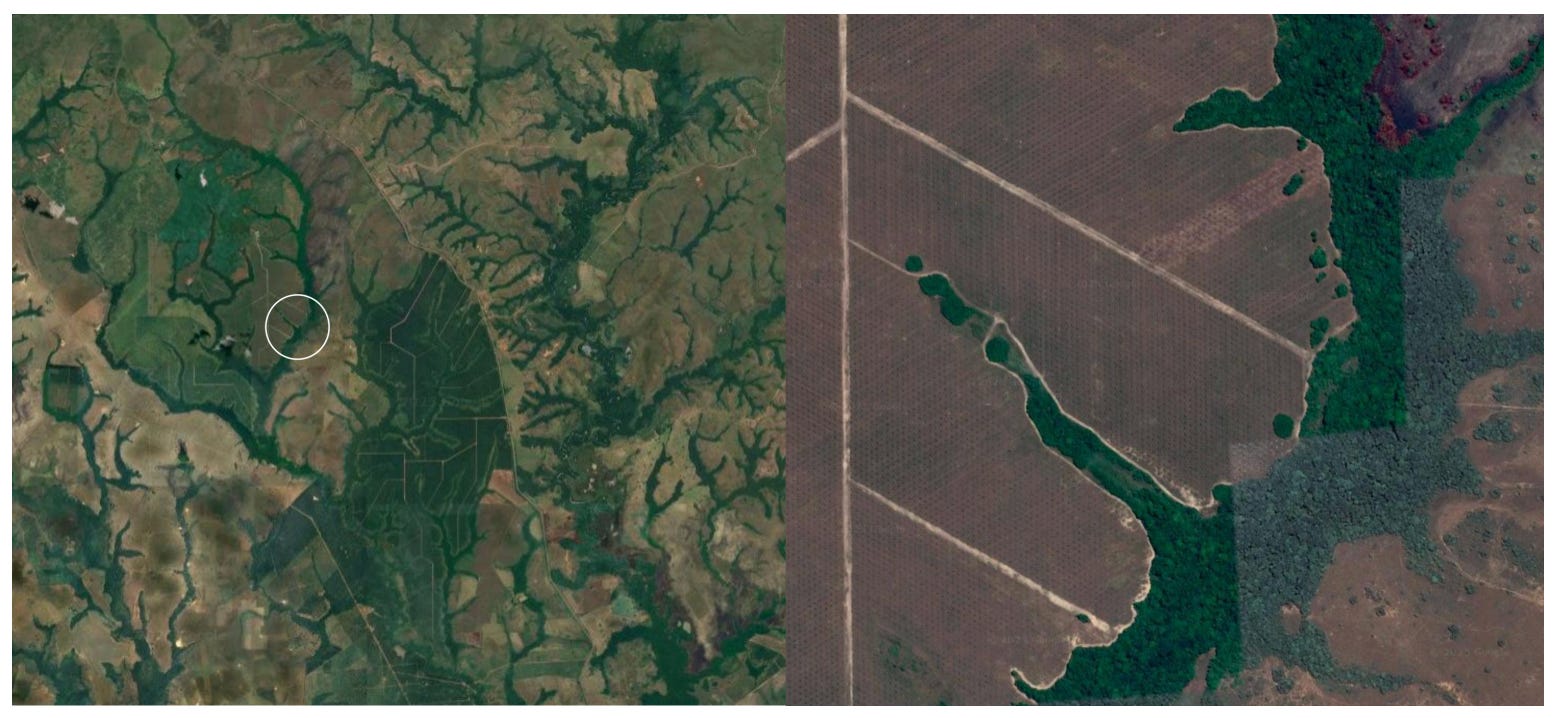
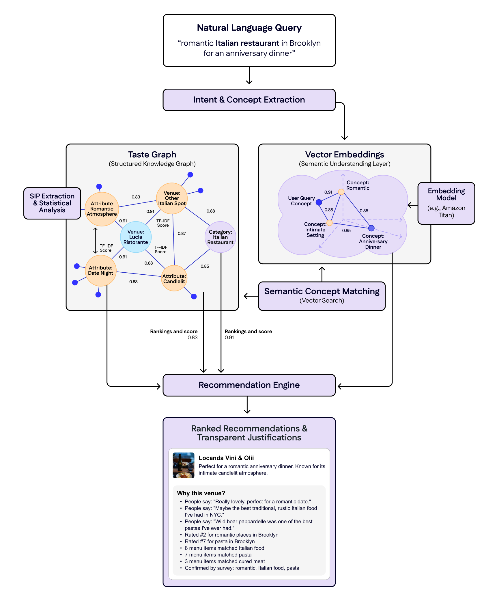


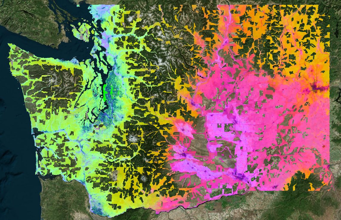

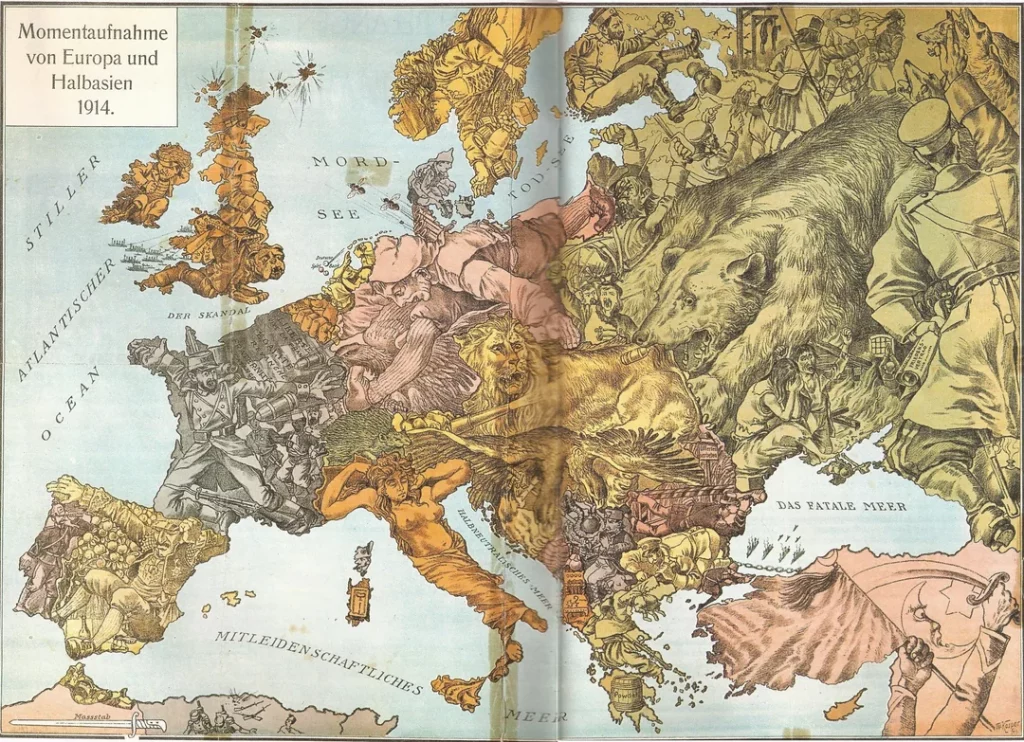

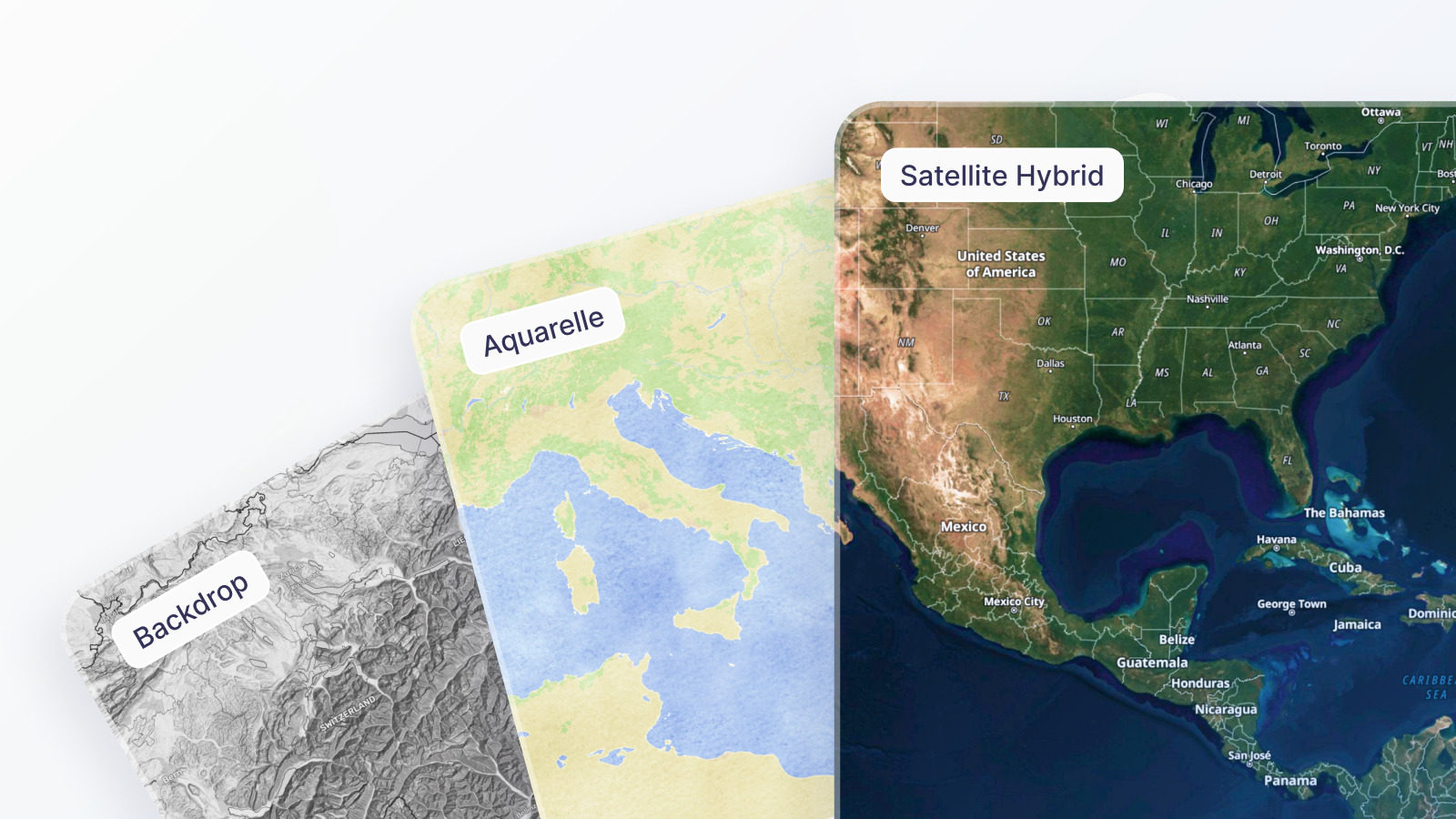


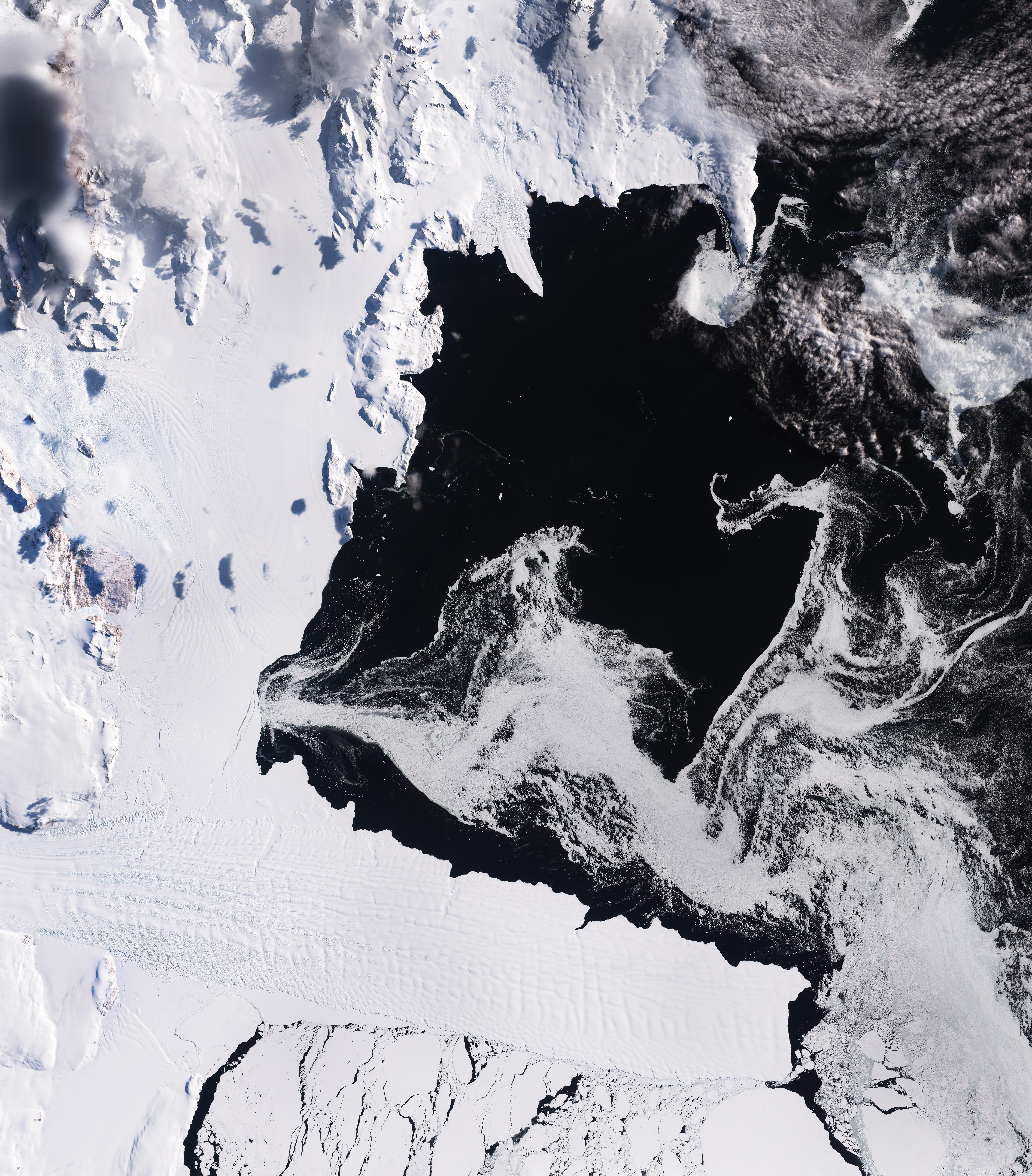


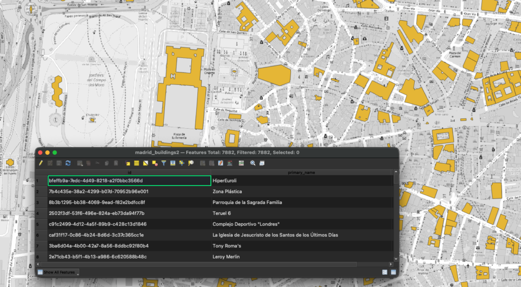
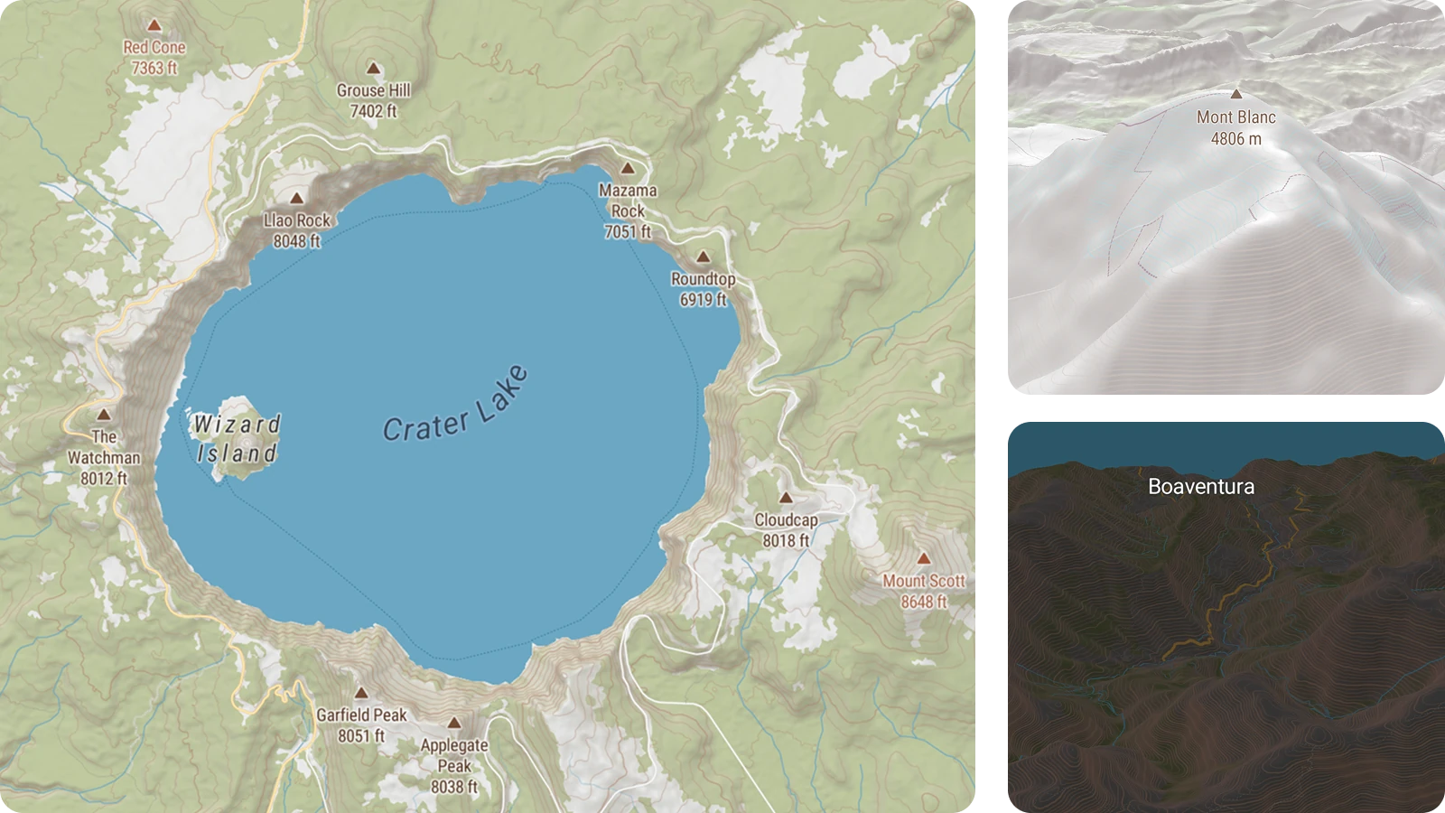

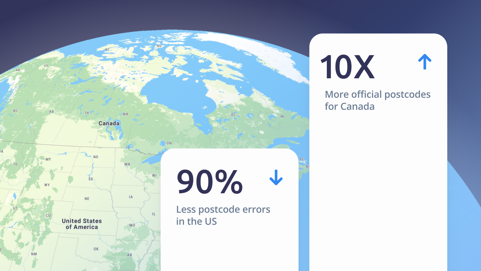


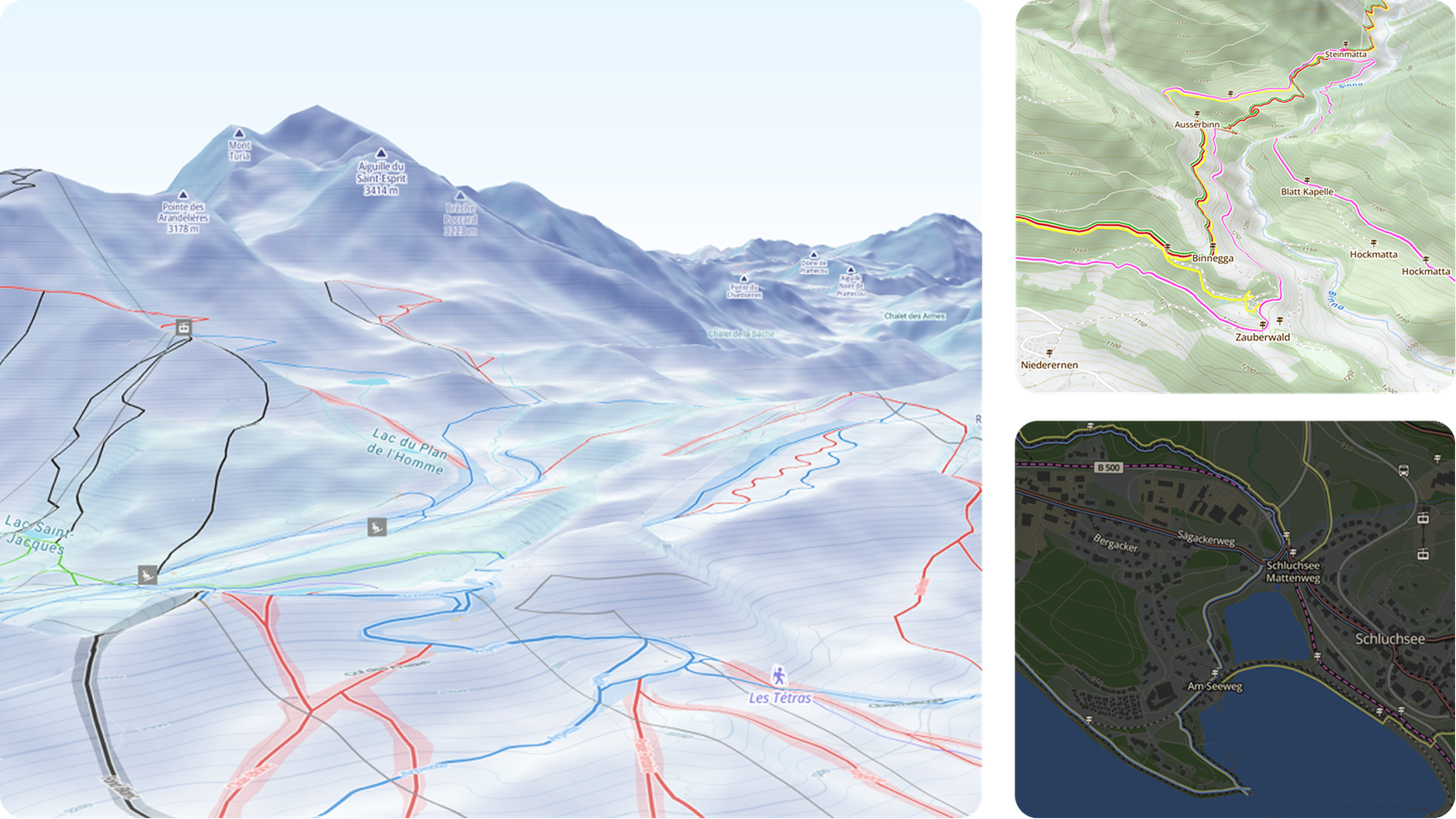


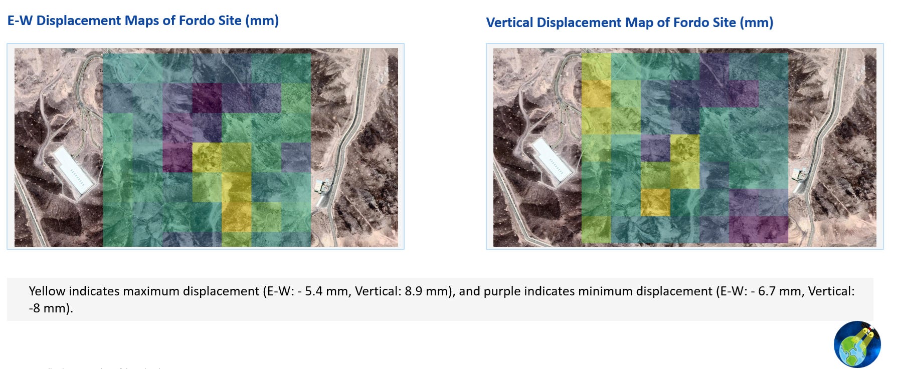
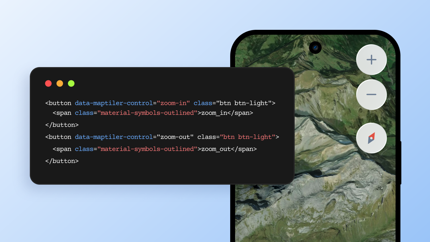

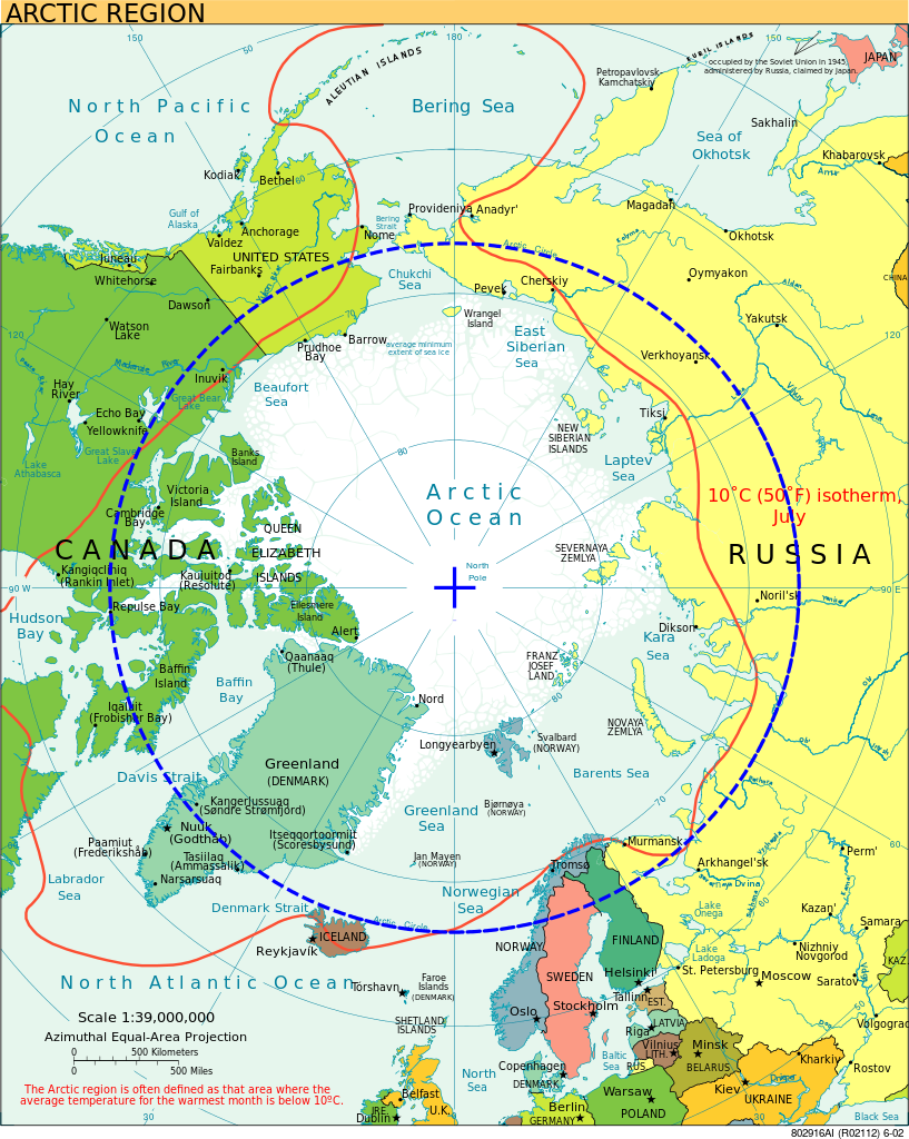


![Oslandia - (Fr) [Équipe Oslandia] Sylvain, GIS Engineer](https://oslandia.com/wp-content/uploads/2026/02/portrait-sylvain.png)
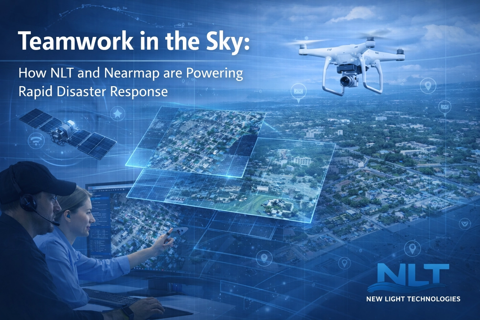


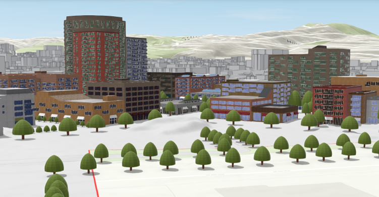
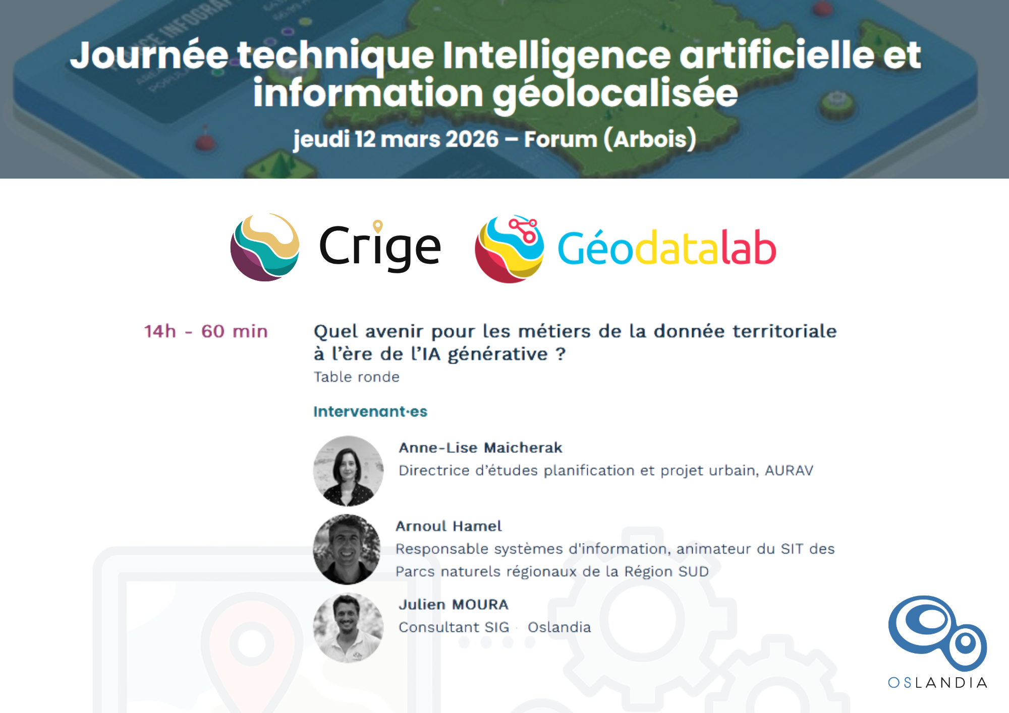


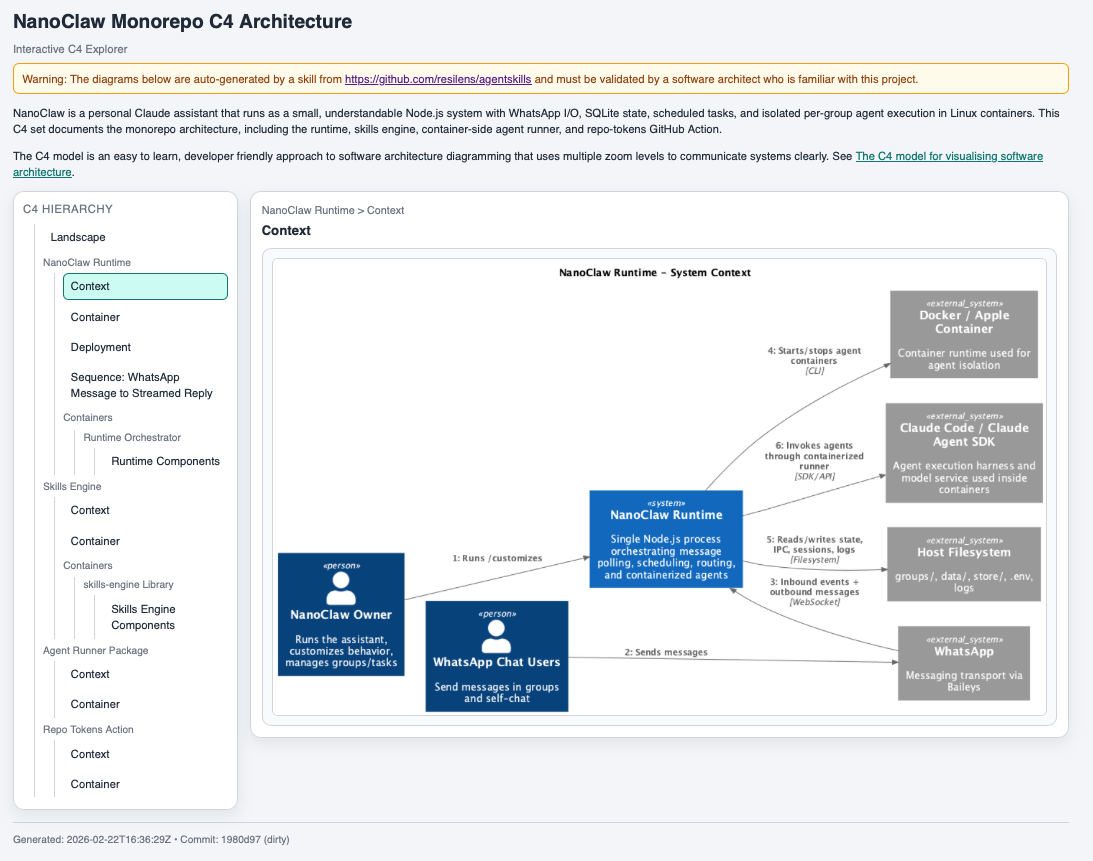


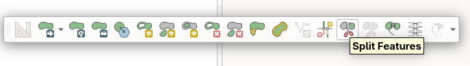


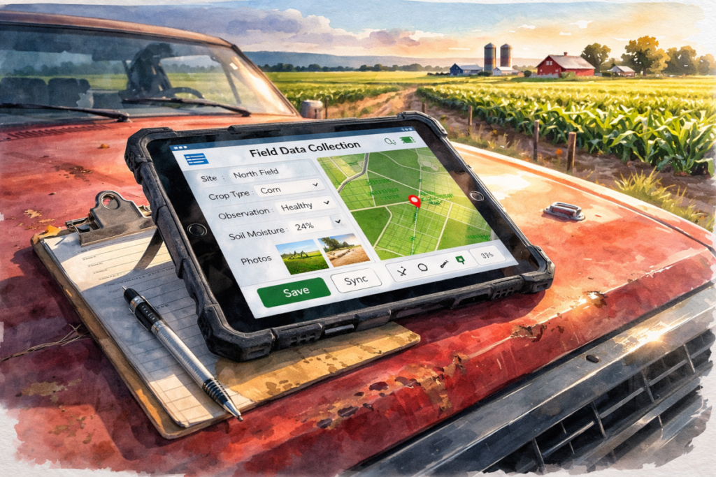
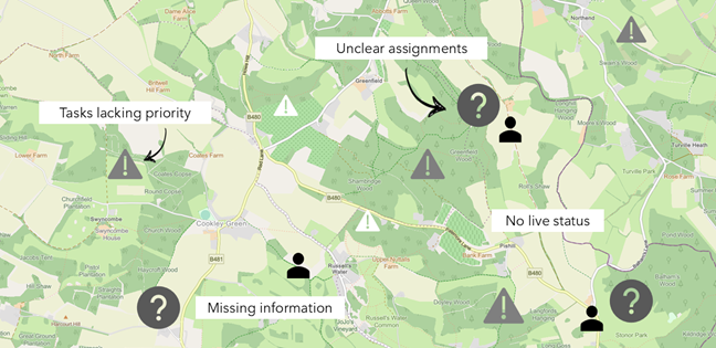


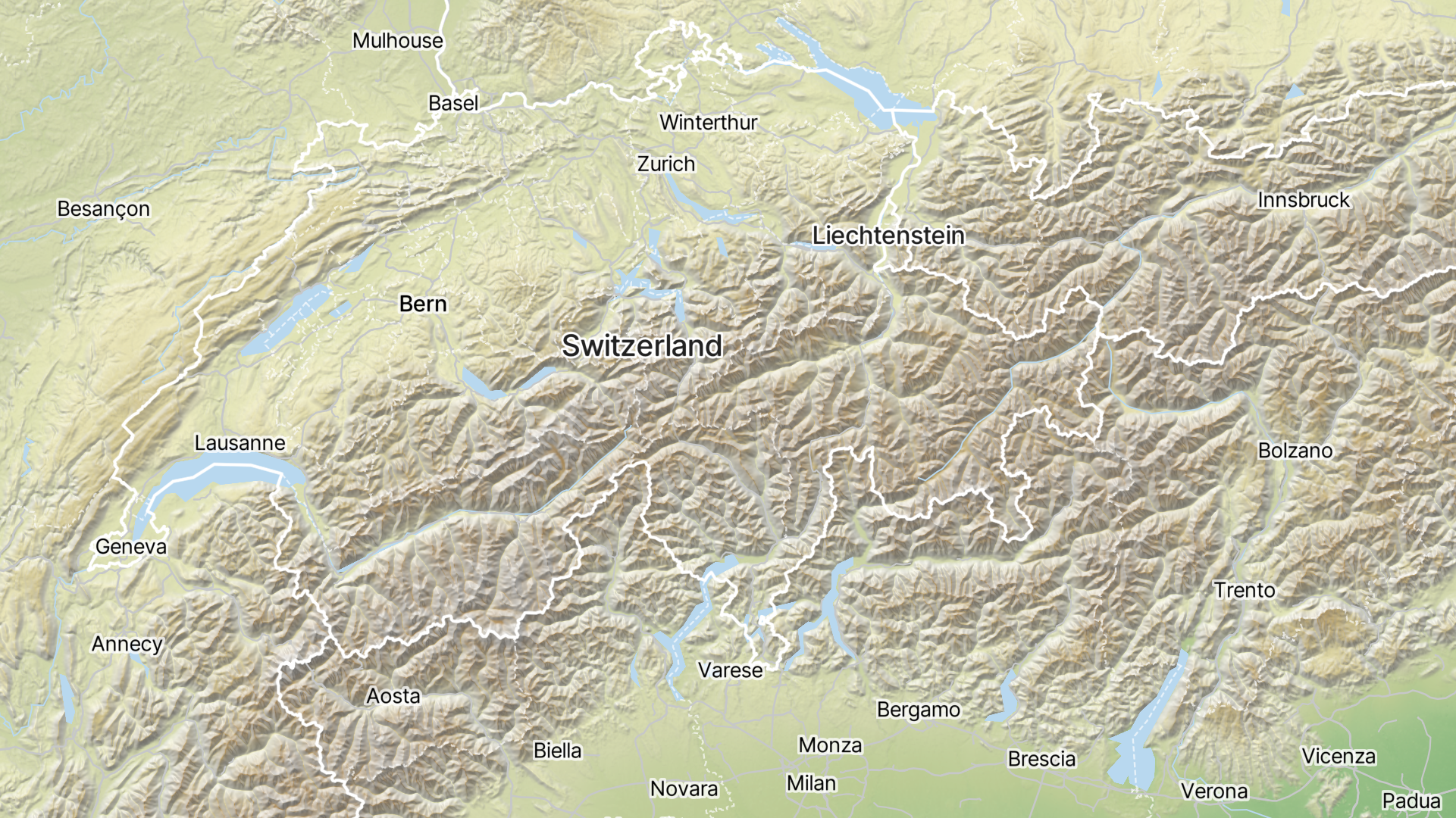


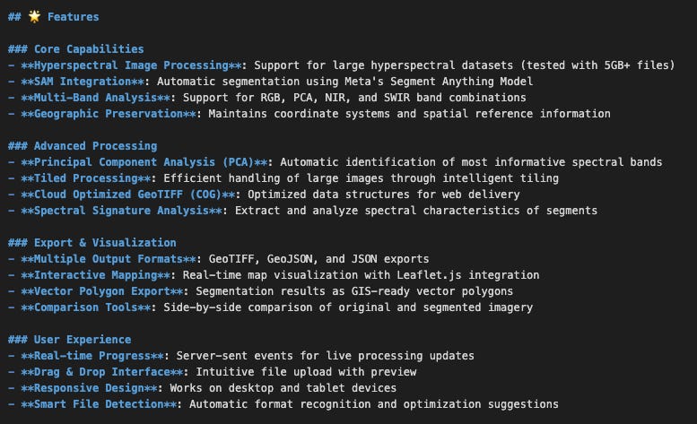

.png)
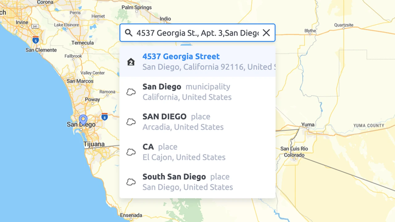
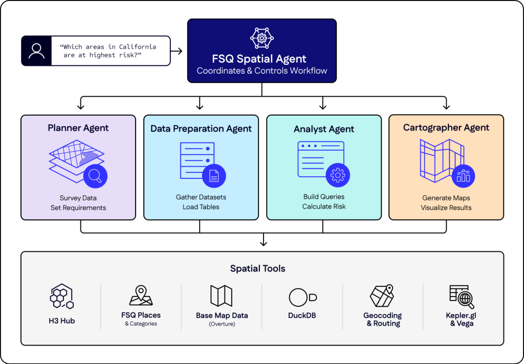


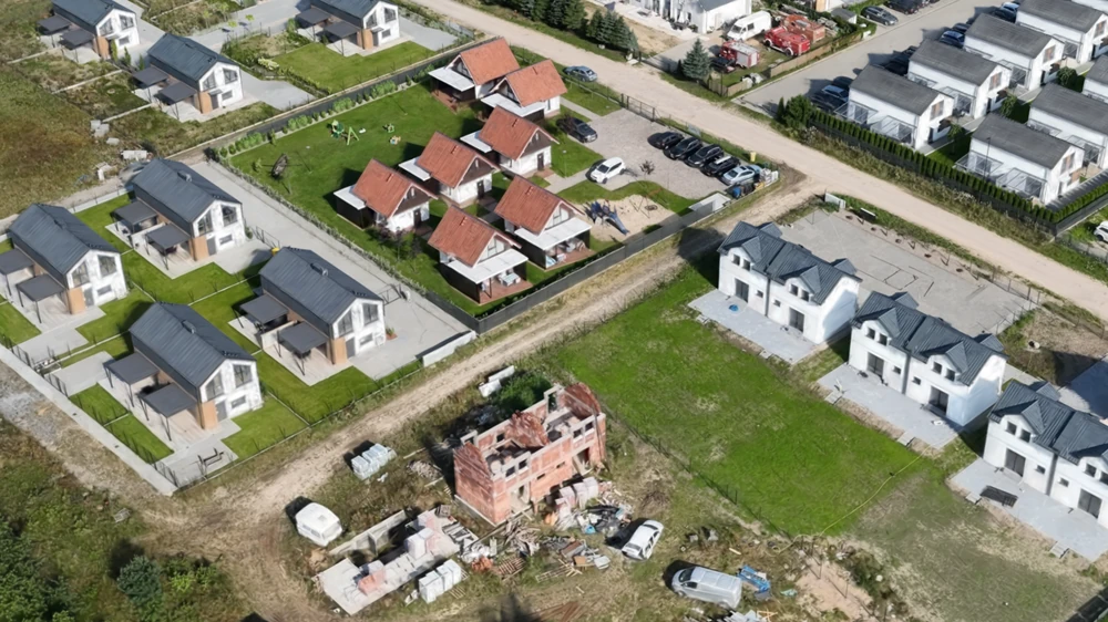

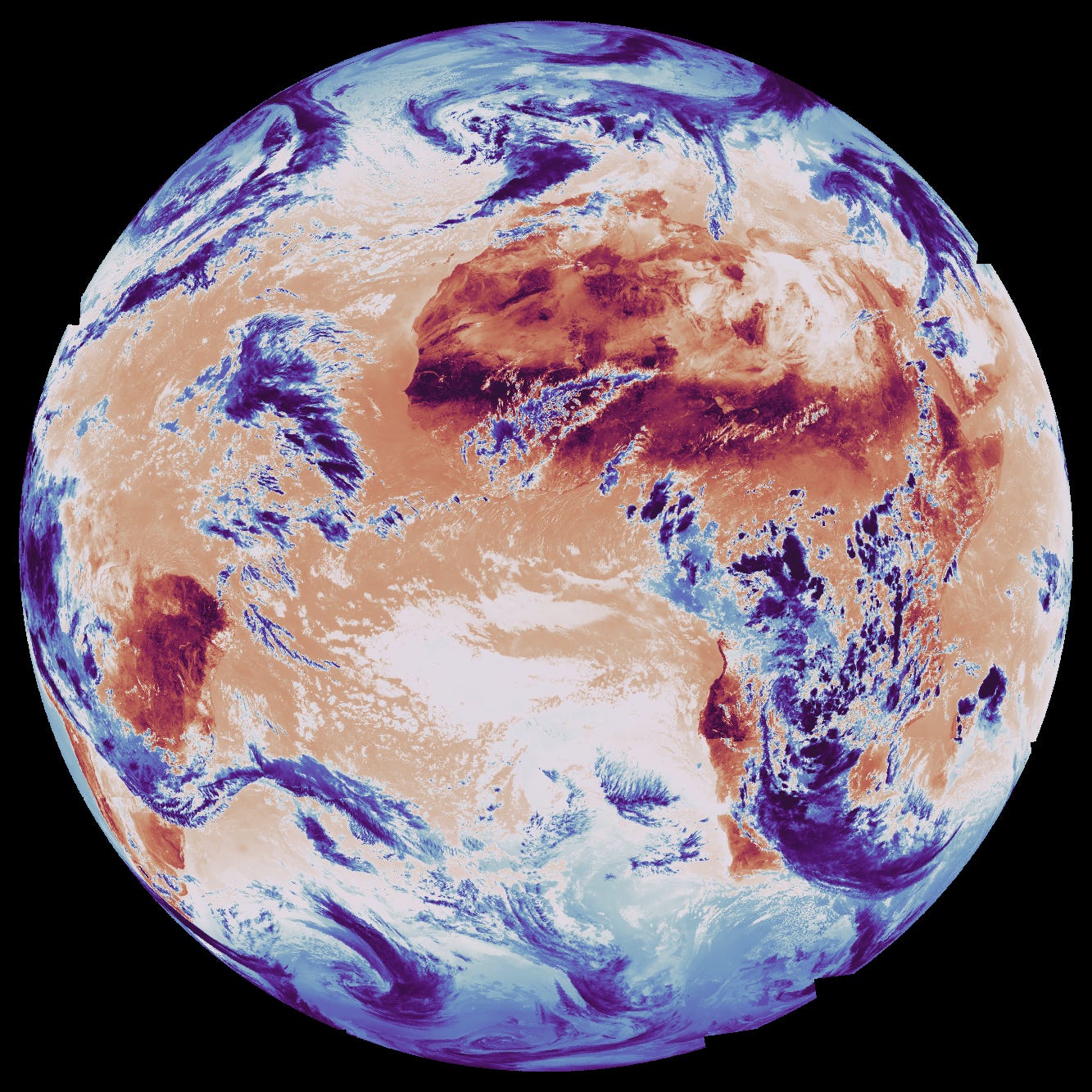
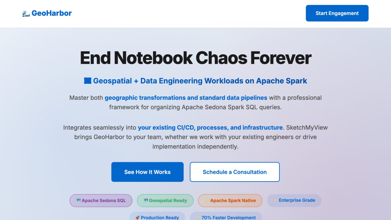


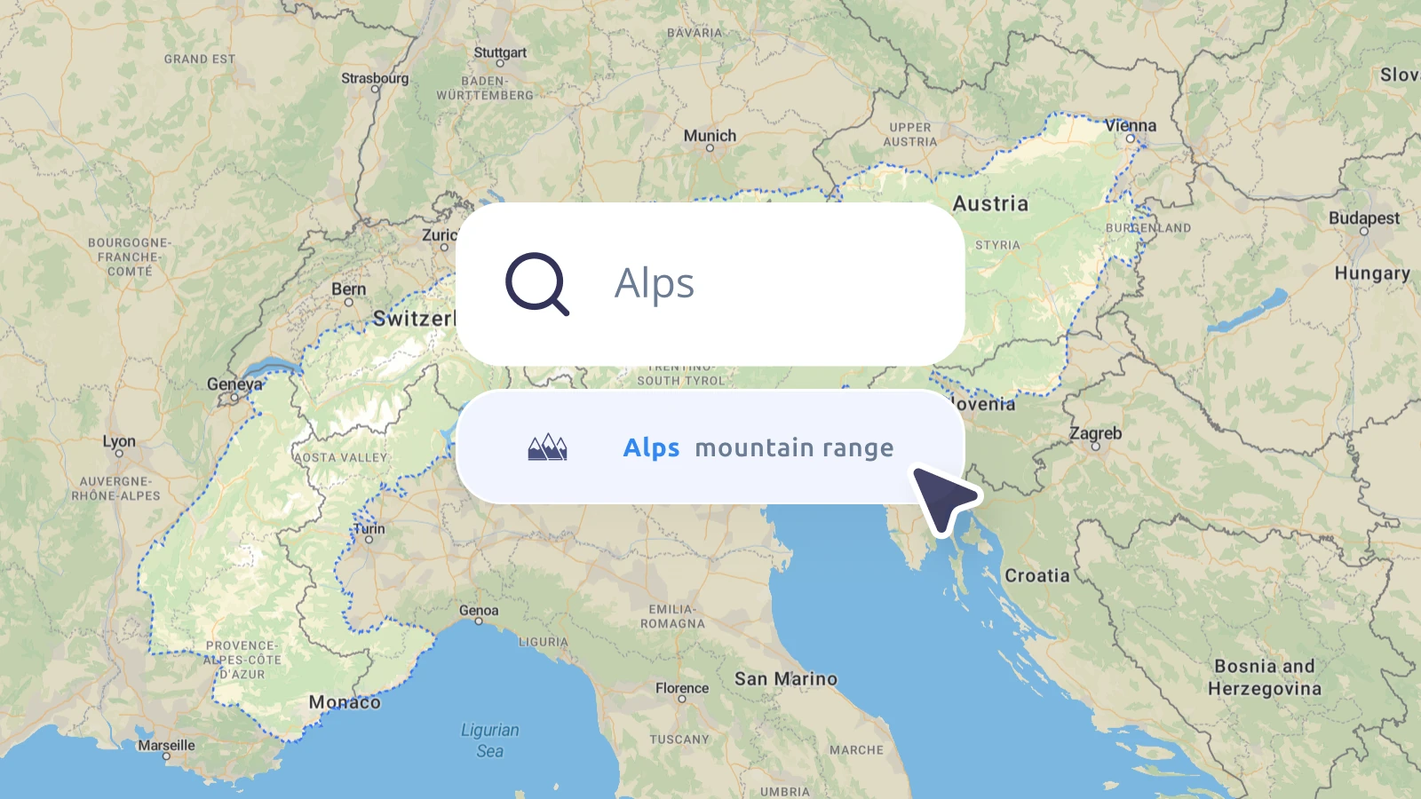
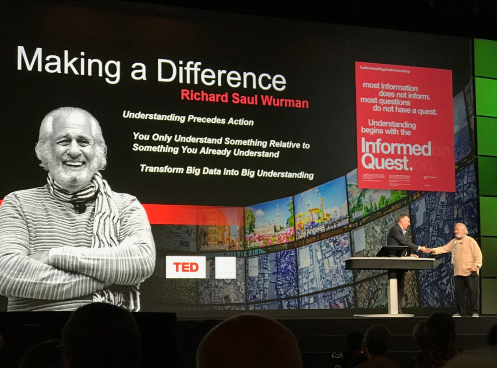
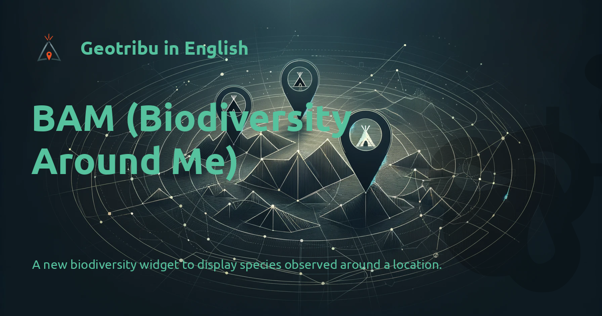
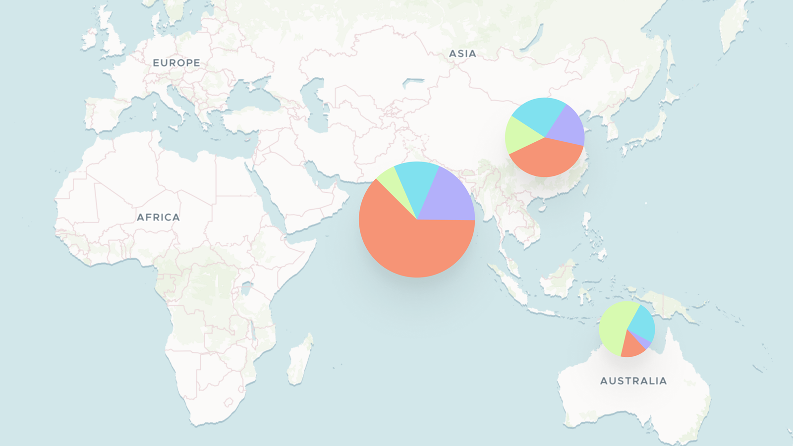


.png?format=1500w)

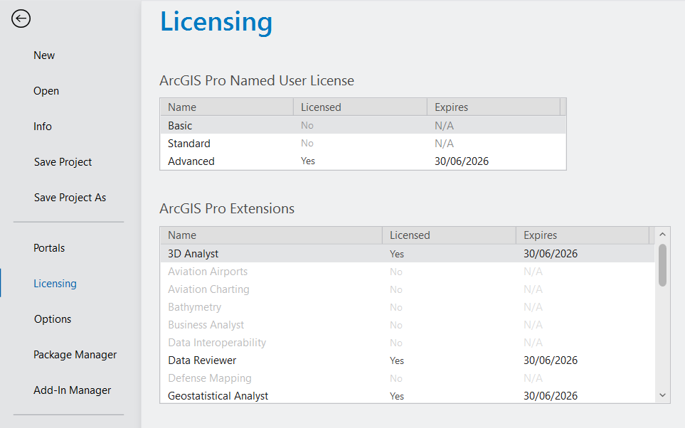
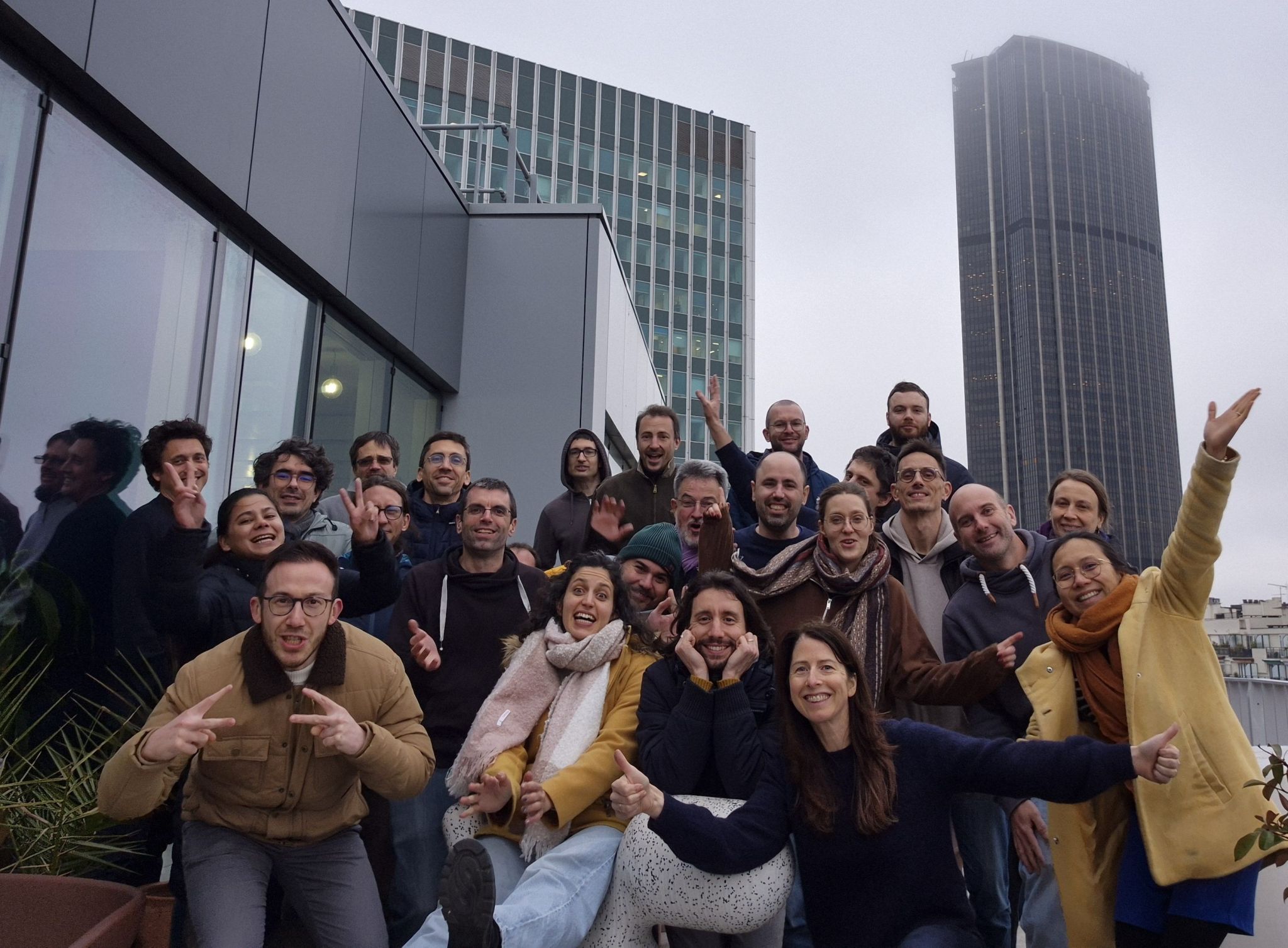


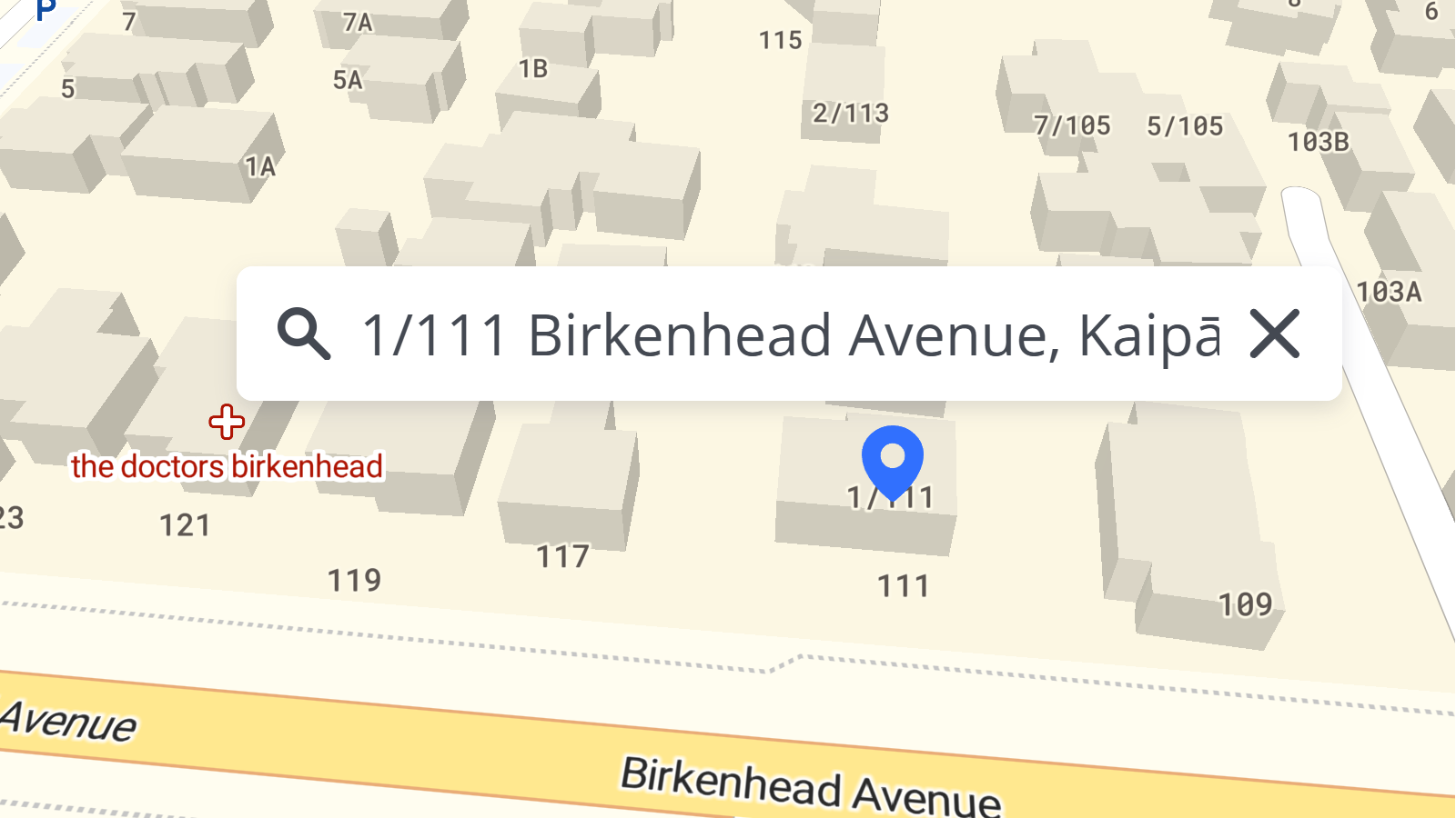

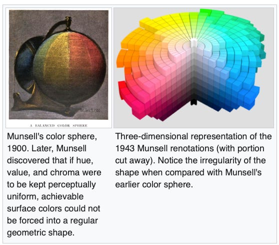

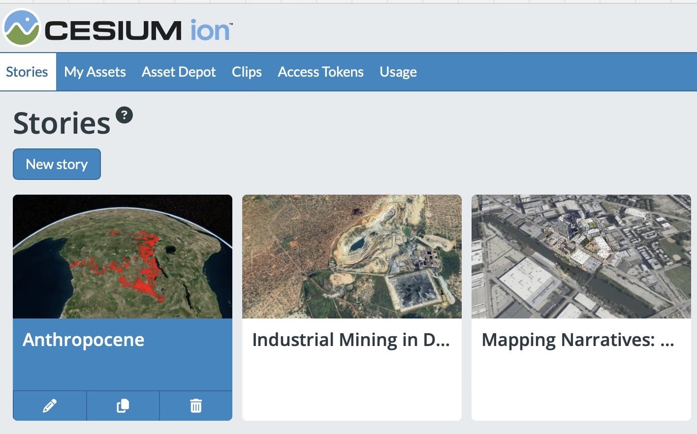

.png?format=1500w)


![Oslandia - (Fr) [Équipe Oslandia] Alicia, assistante administrative et comptable](https://oslandia.com/wp-content/uploads/2025/12/portrait-alicia.png)
![Mergin Maps blog - [QGIS] Plugin and API update brings simultaneous syncs](https://cdn.prod.website-files.com/64be358a4fb0e612b228bb9e/697b875f167560ff1d3d0f23_Image%2024.jpg)

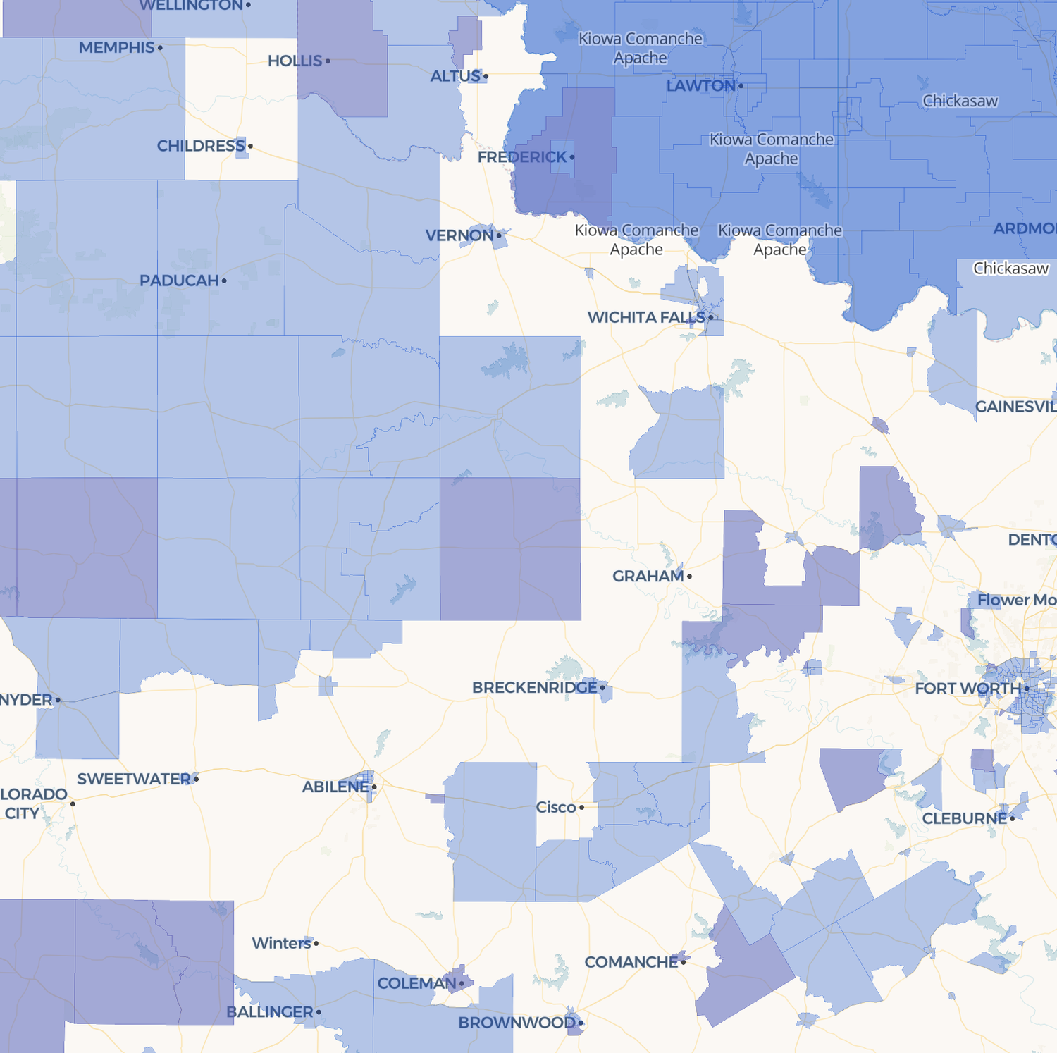


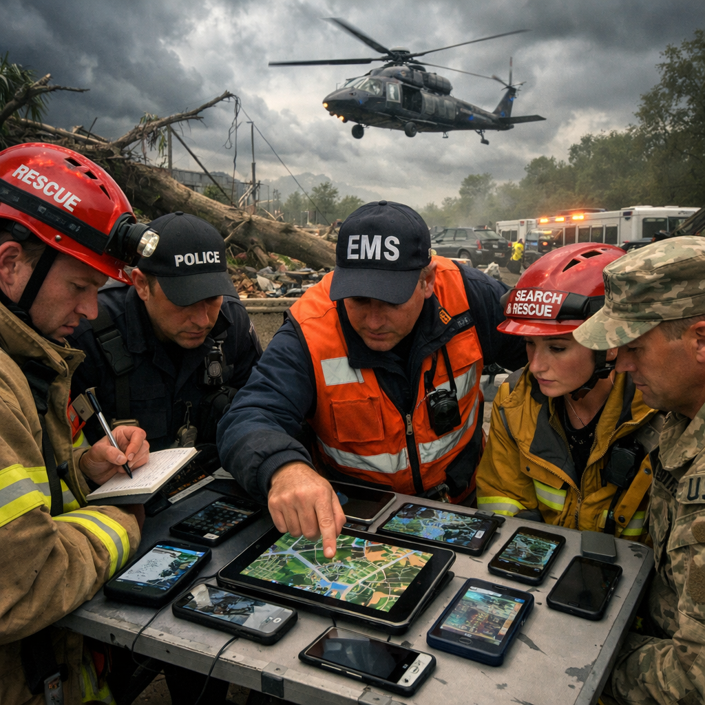


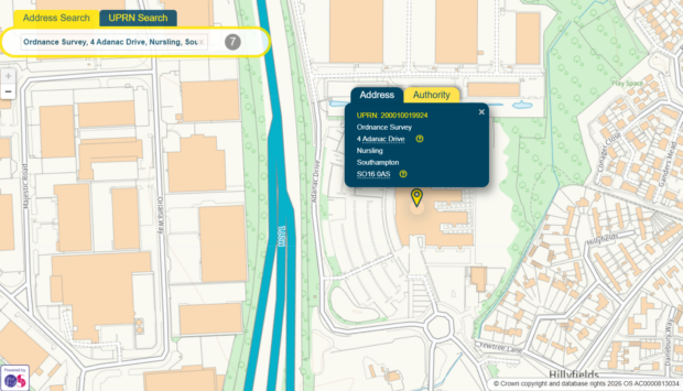

![Mergin Maps blog - [QGIS] How to import geotagged photos into QGIS for fieldwork mapping](https://cdn.prod.website-files.com/64be358a4fb0e612b228bb9e/697390d970d3c710efb9761d_unnamed%20(8)(1).png)

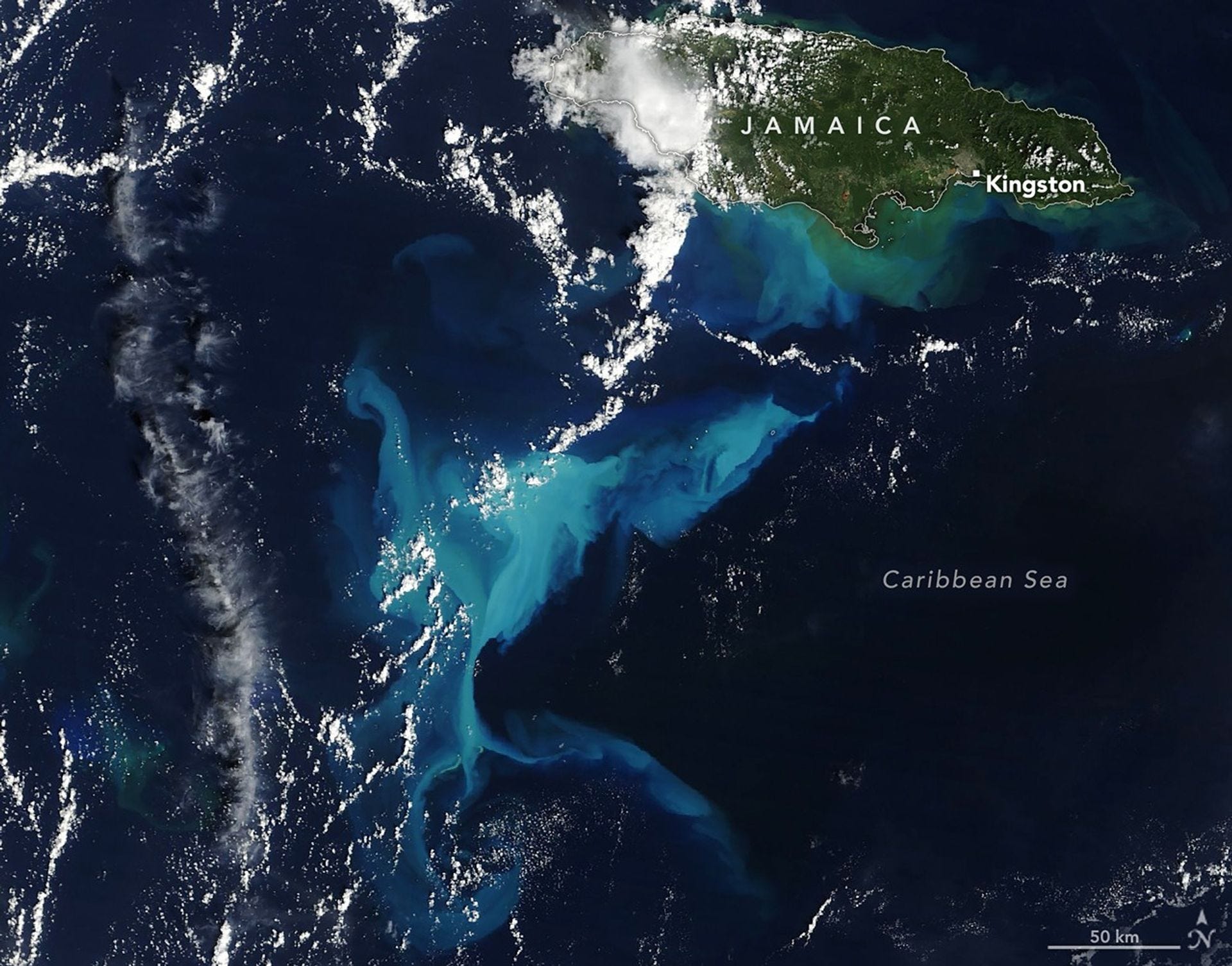


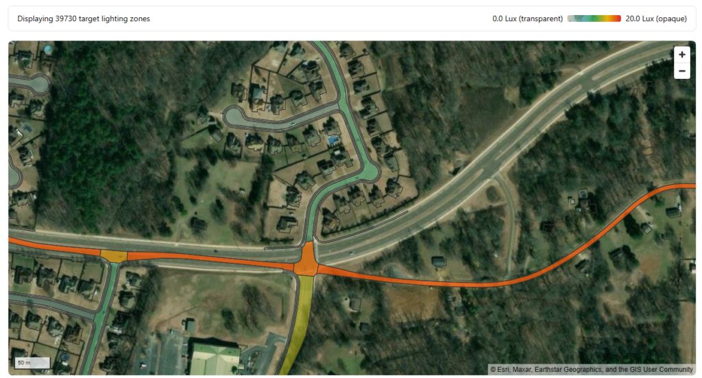


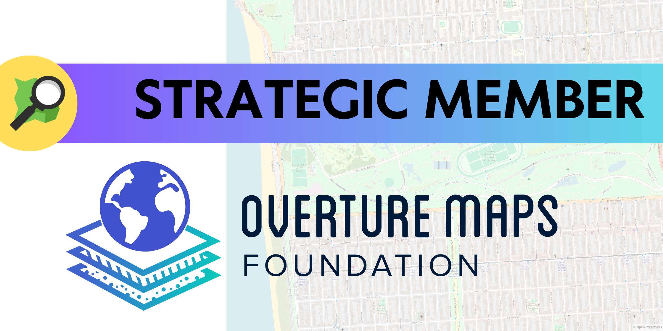
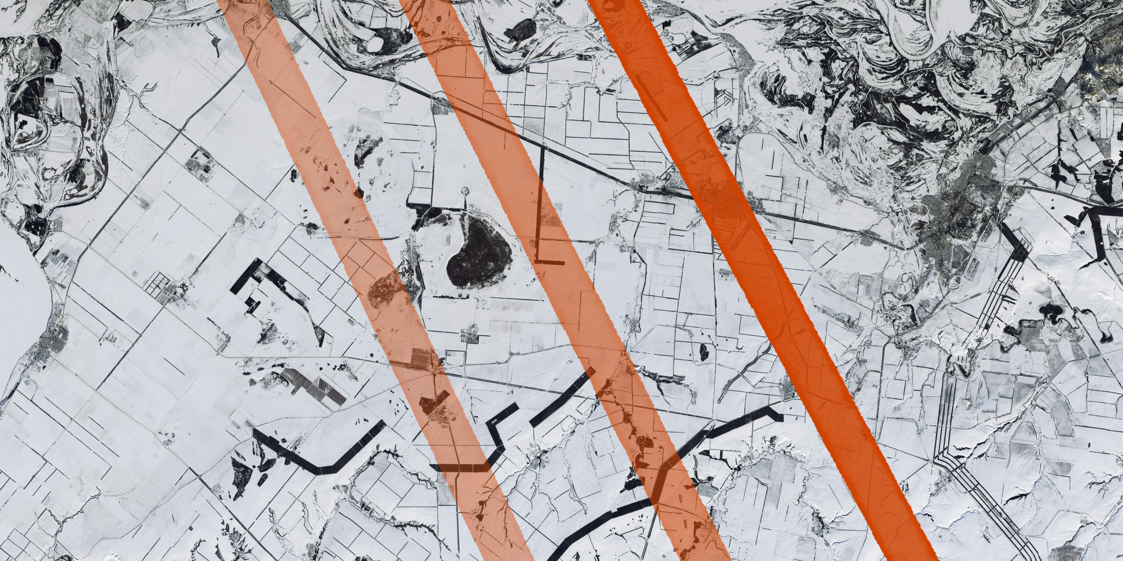

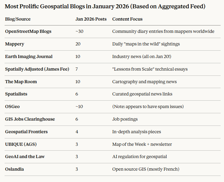
![Oslandia - (Fr) [Témoignage client] Nourredine Idir, AURCA](https://oslandia.com/wp-content/uploads/2025/12/t%C3%A9moignage-nourredine-idir.png)
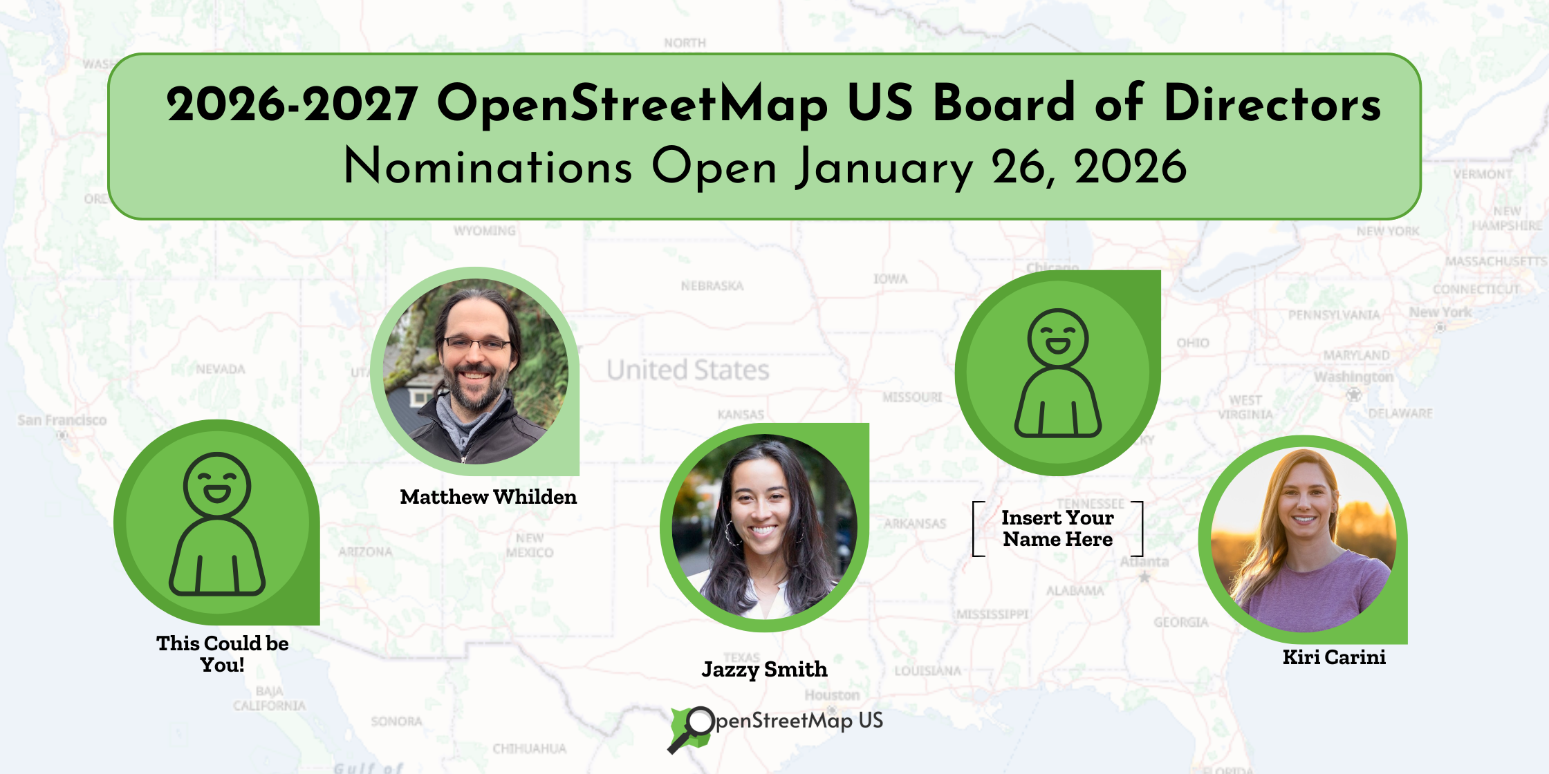
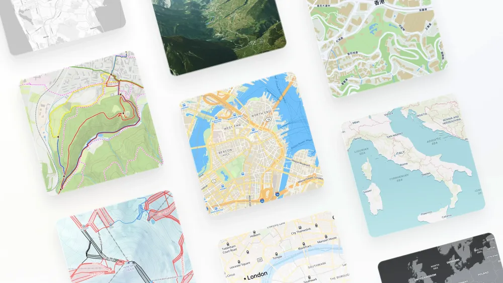


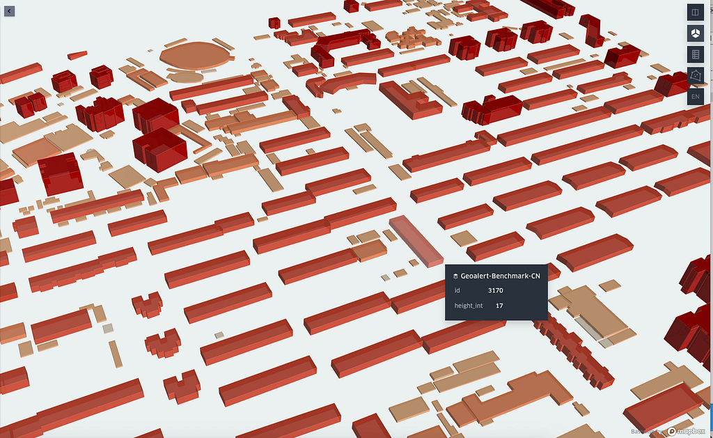


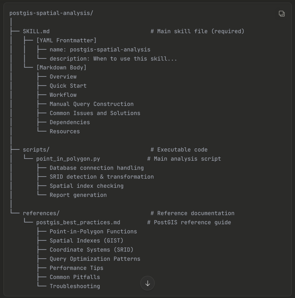
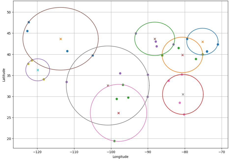


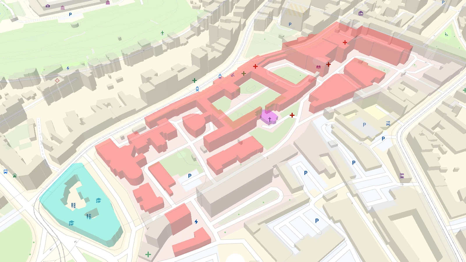


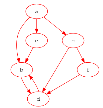
![Mergin Maps case studies - [QGIS] Open source geological mapping with British Geological Survey](https://cdn.prod.website-files.com/64be358a4fb0e612b228bb9e/695f88b19d3f4a1405ddf69c_20231024_151205.jpg)

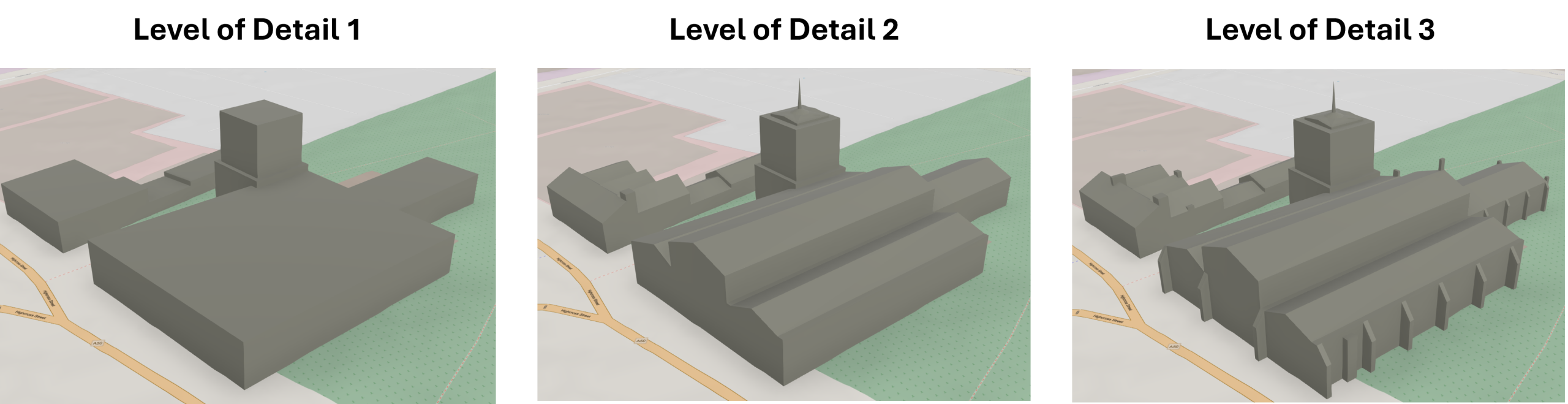

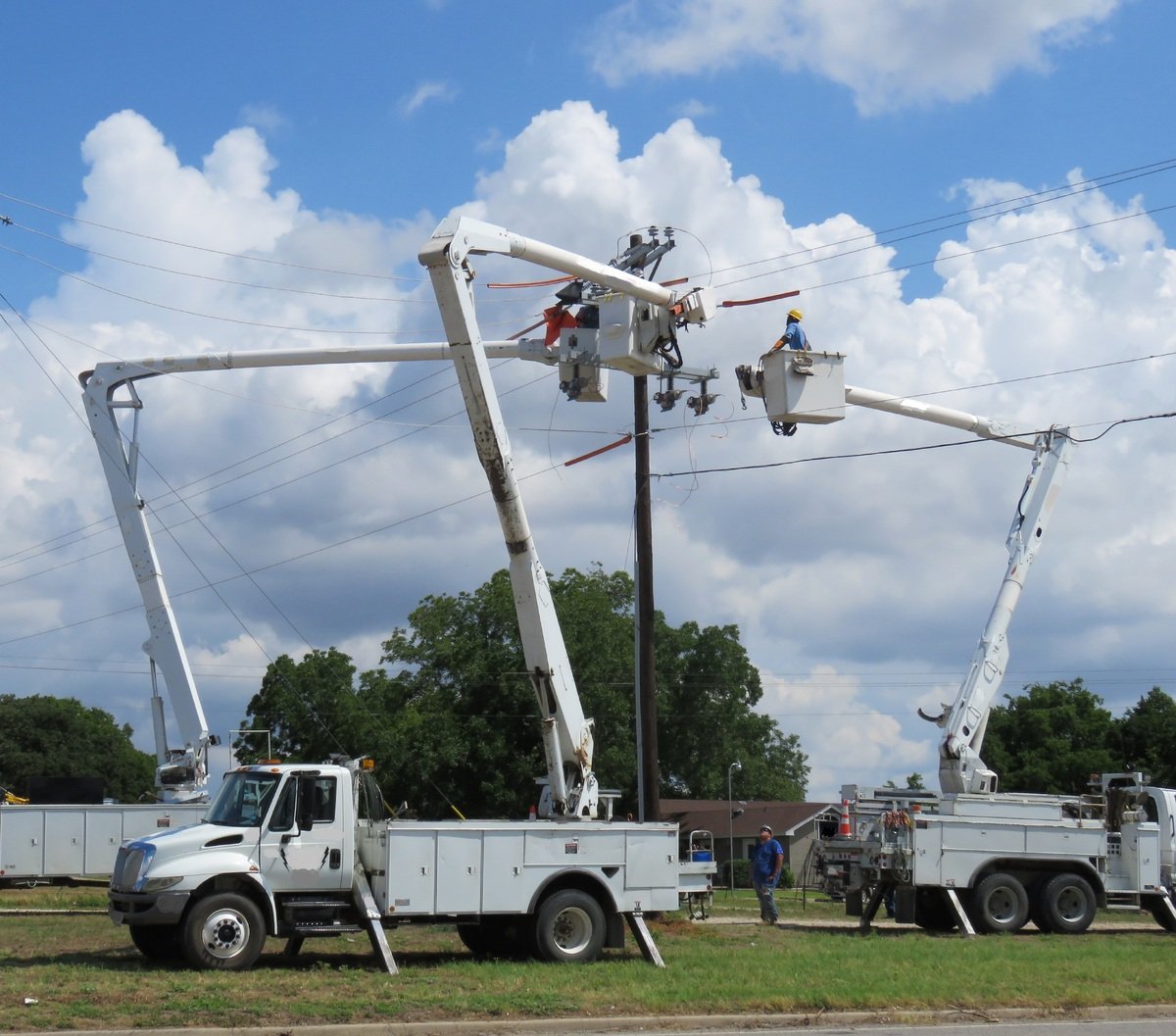


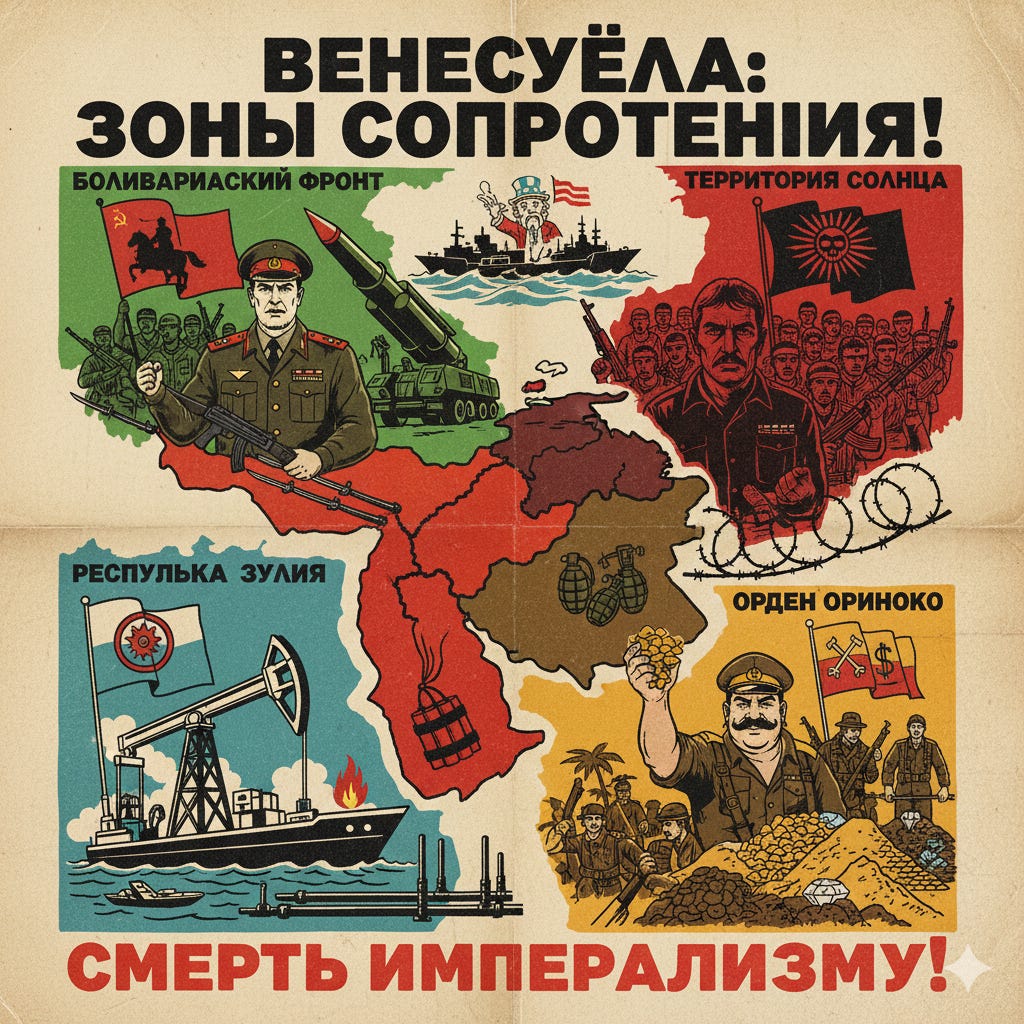


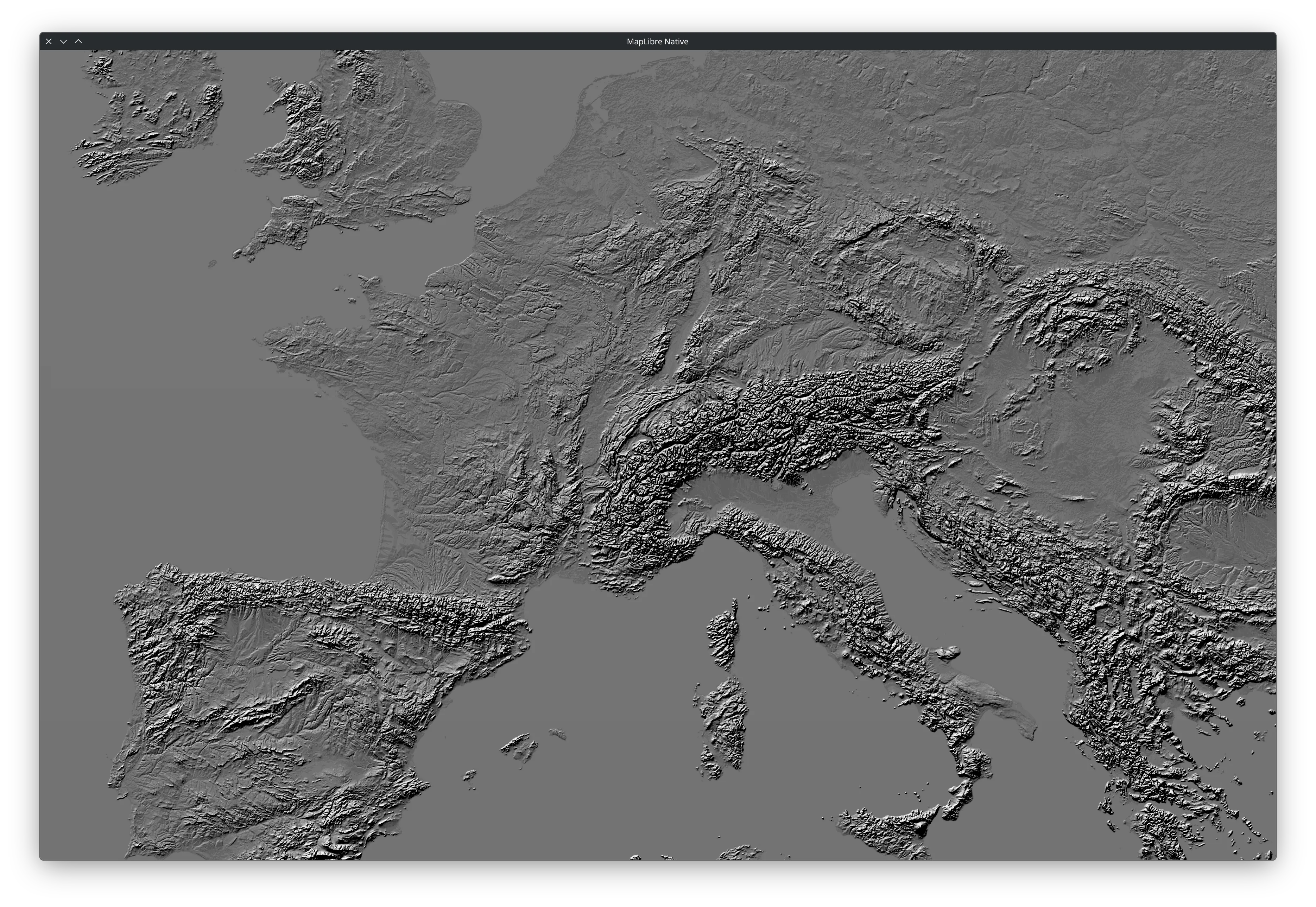

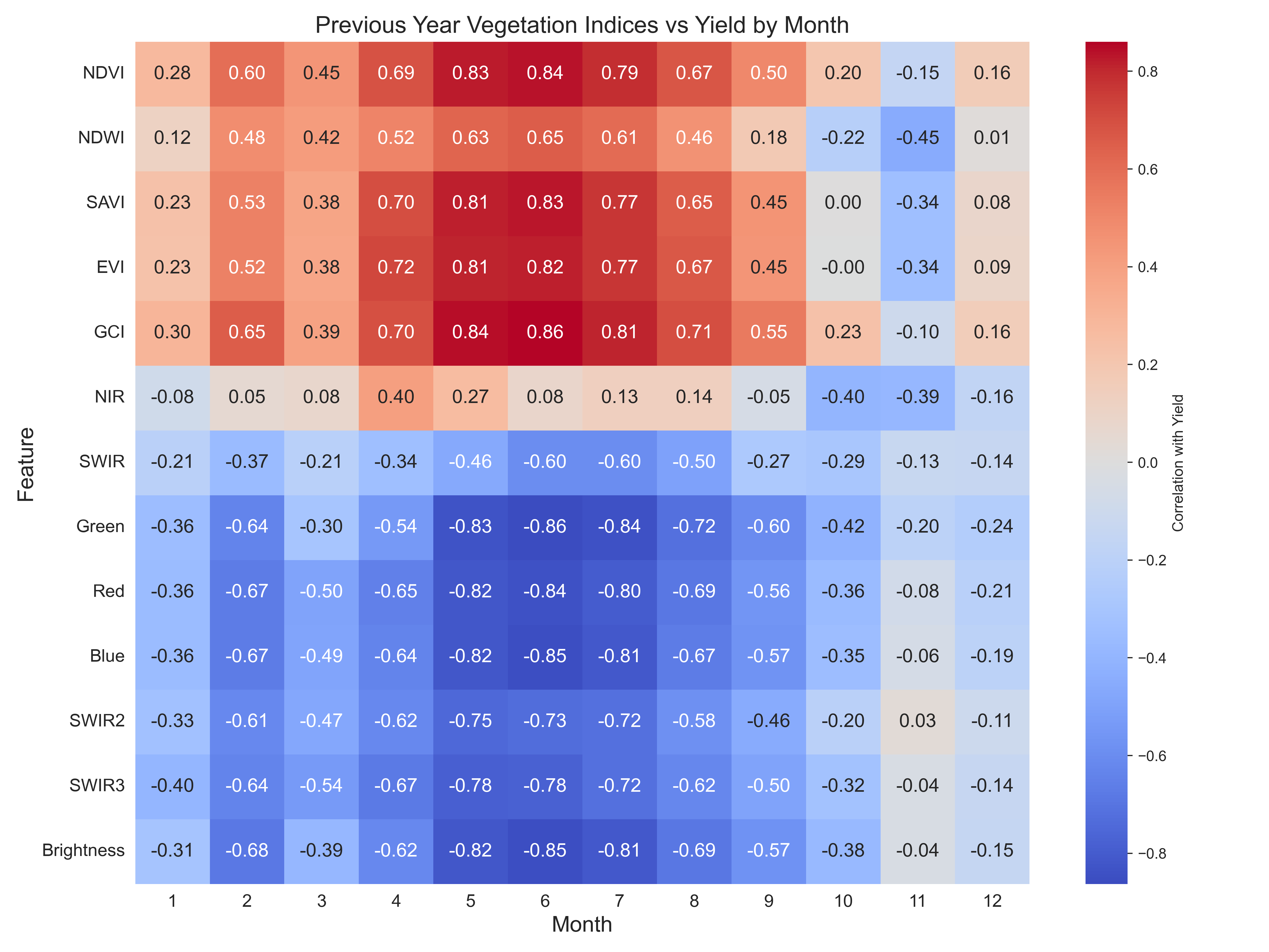
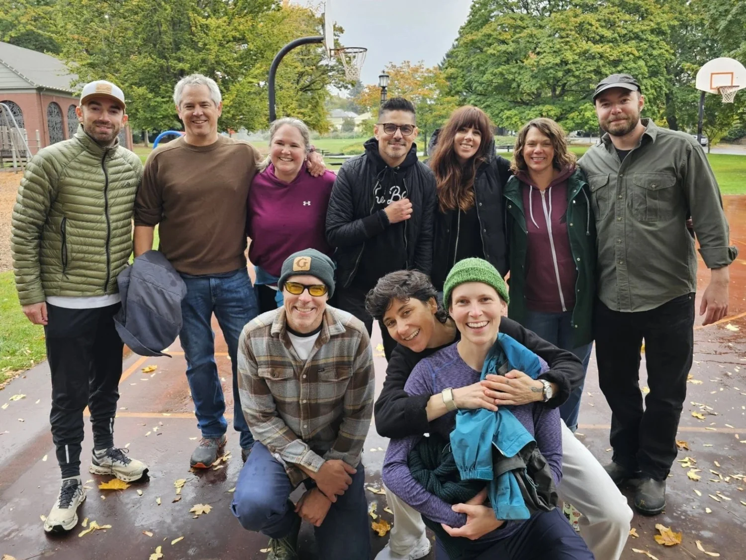
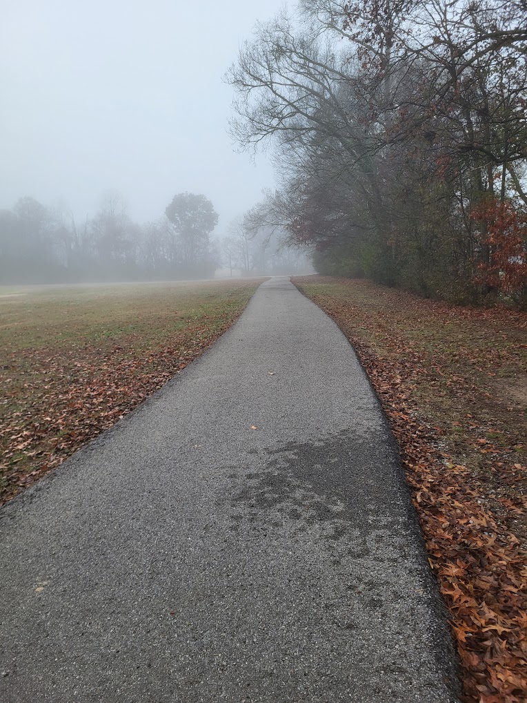
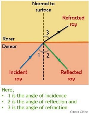

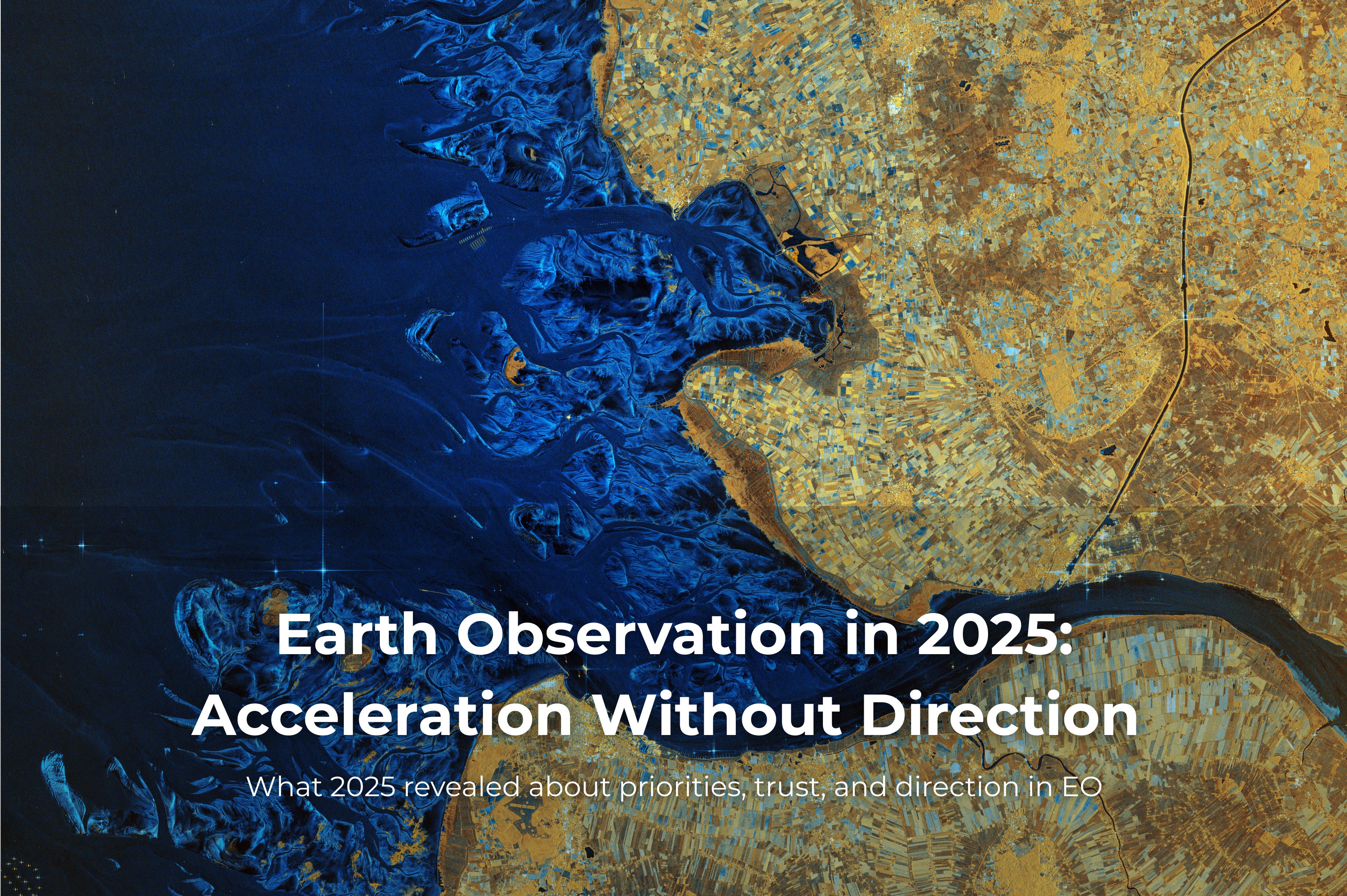


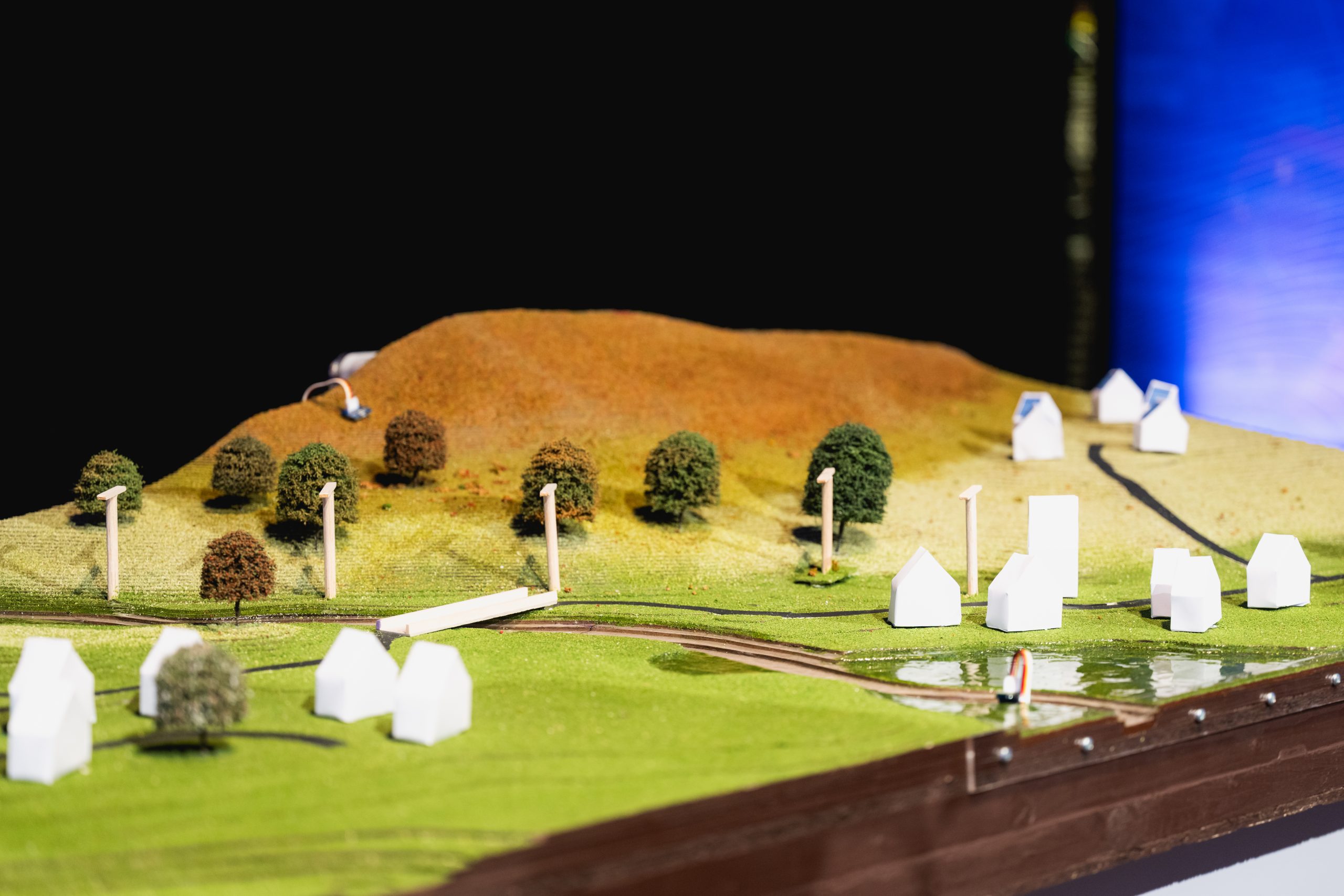


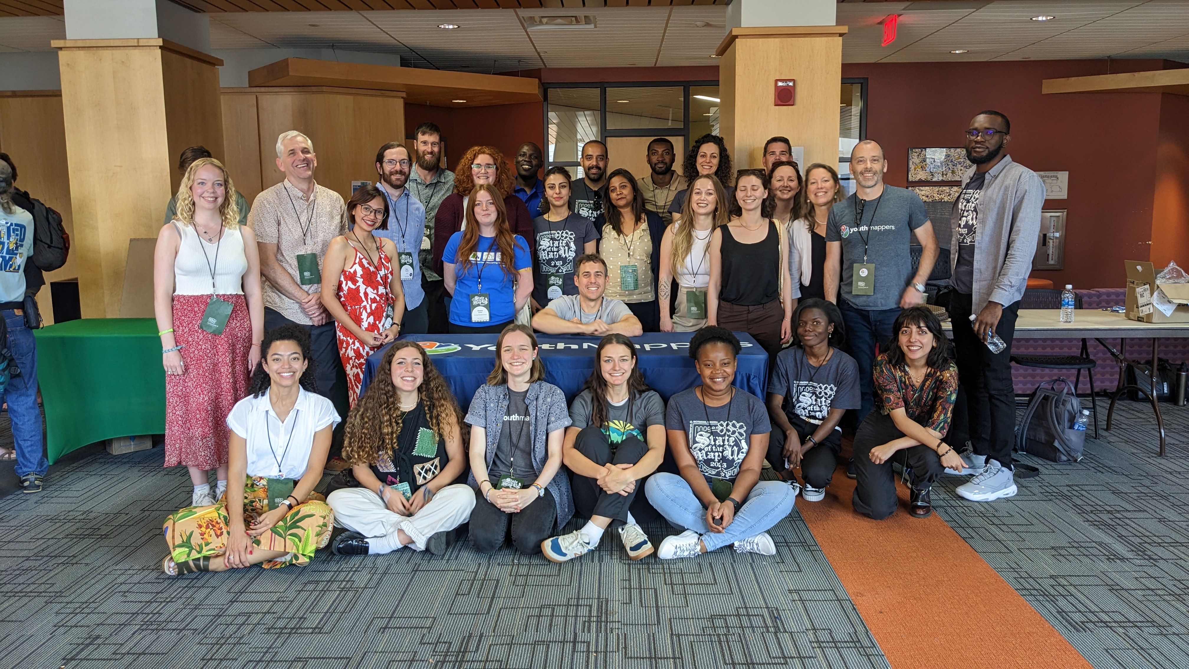
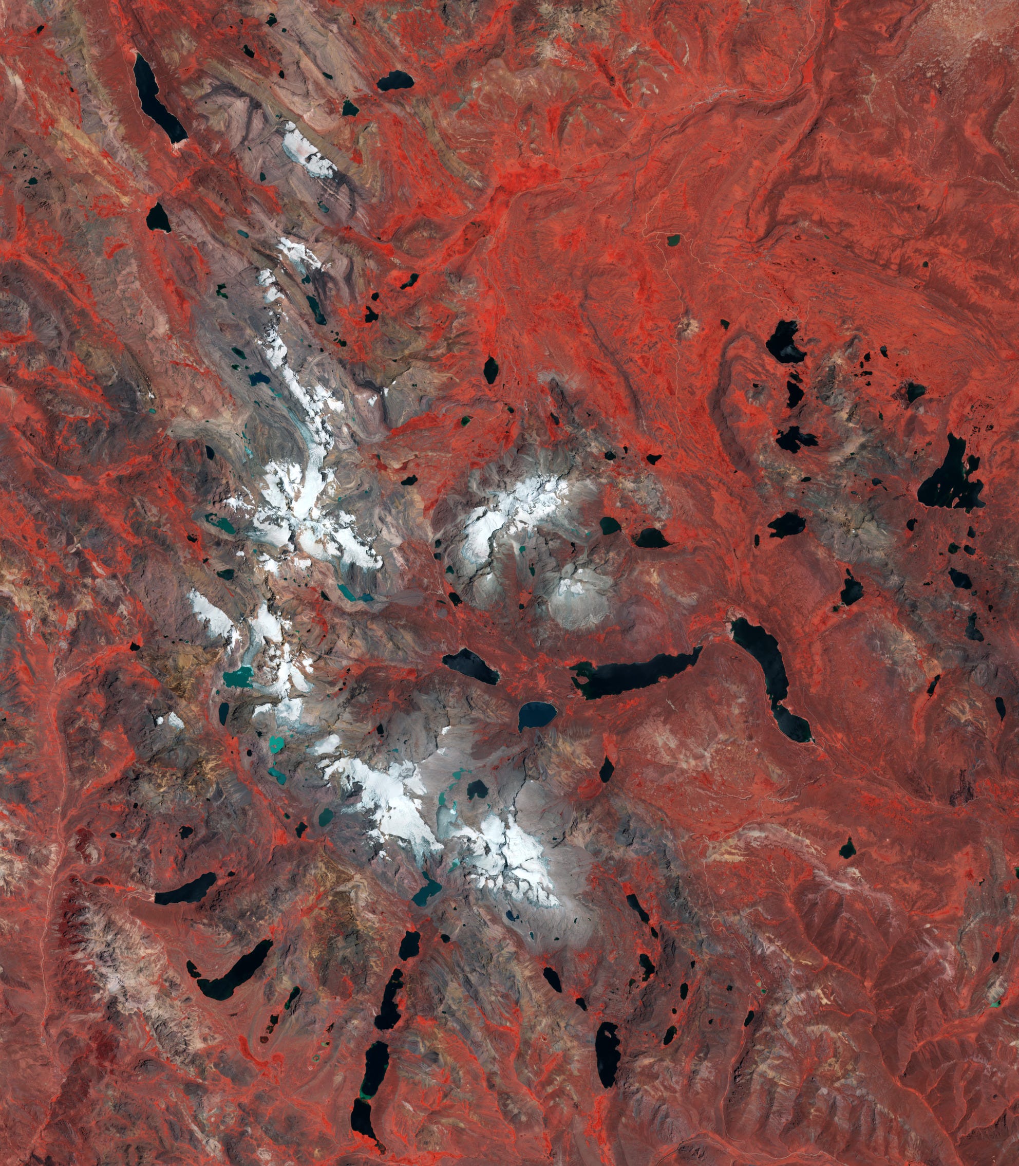


![Oslandia - (Fr) [Équipe Oslandia] Jérémy Garniaux, Doctorant CIFRE en archéologie numérique et développeur SIG à Oslandia](https://oslandia.com/wp-content/uploads/2025/11/portrait-j%C3%A9r%C3%A9my.png)


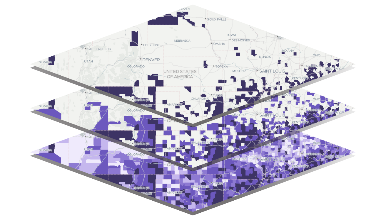

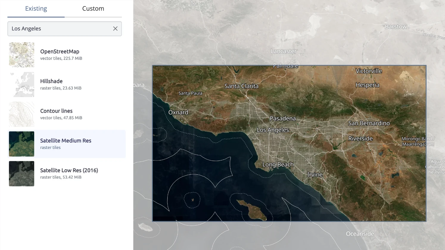


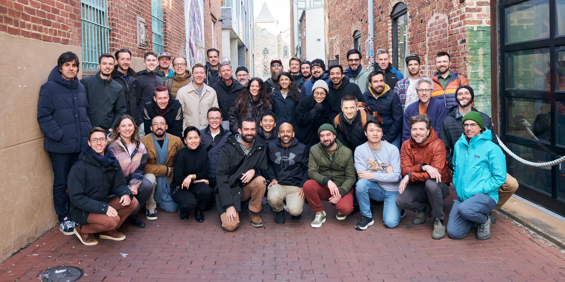
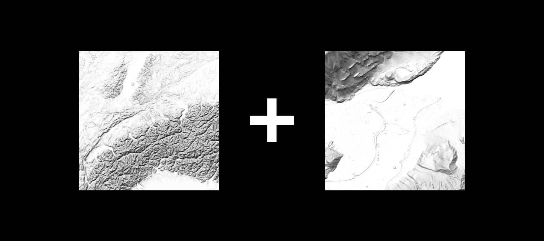

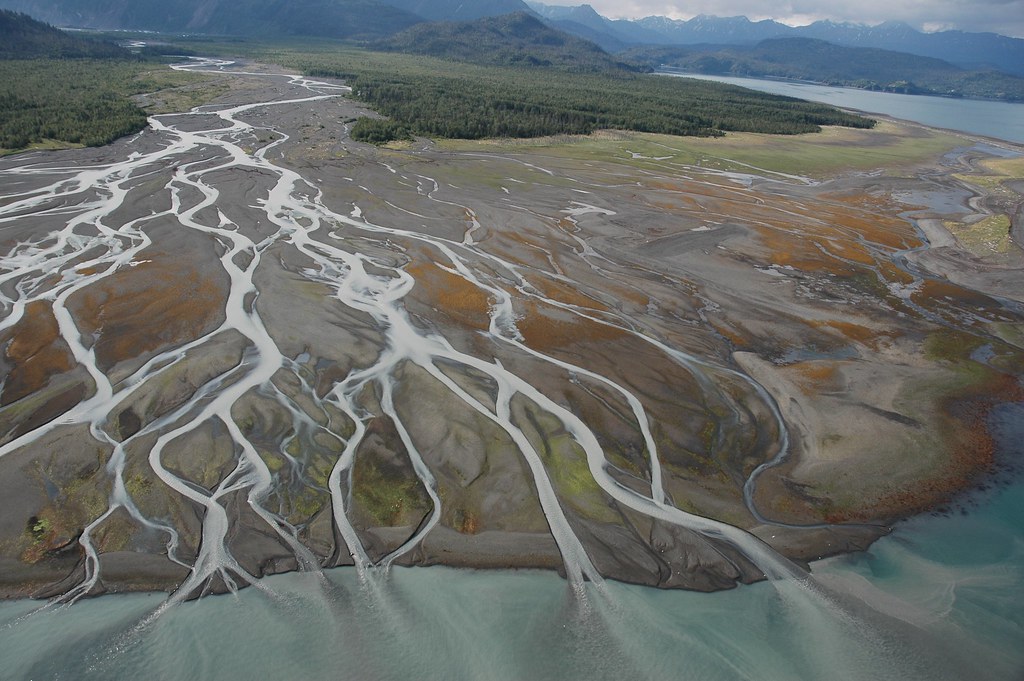
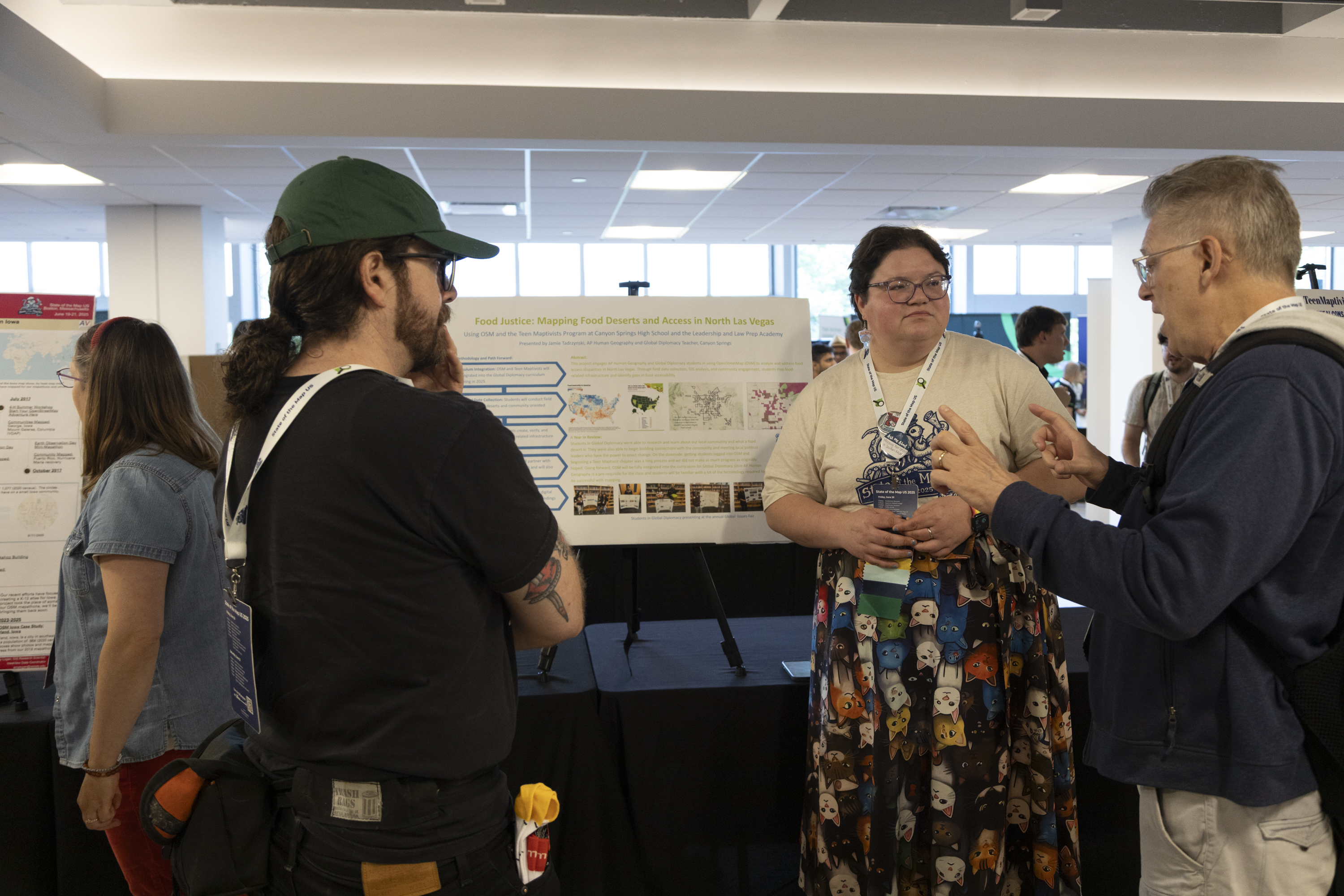
![Mergin Maps blog - [QGIS] Share maps via URL: now in early access](https://cdn.prod.website-files.com/64be358a4fb0e612b228bb9e/694004ee1d8b1b55f7df9b19_69290d04a9518f5b407563a47a6b414a(1).png)
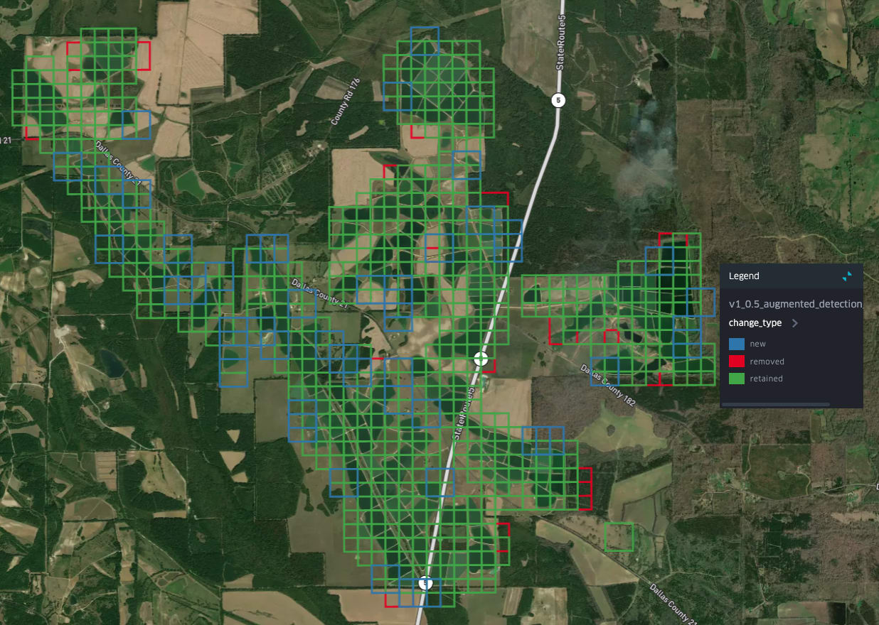
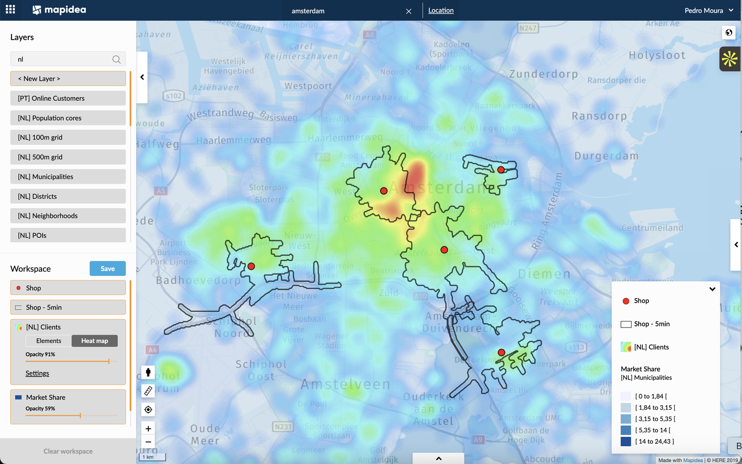
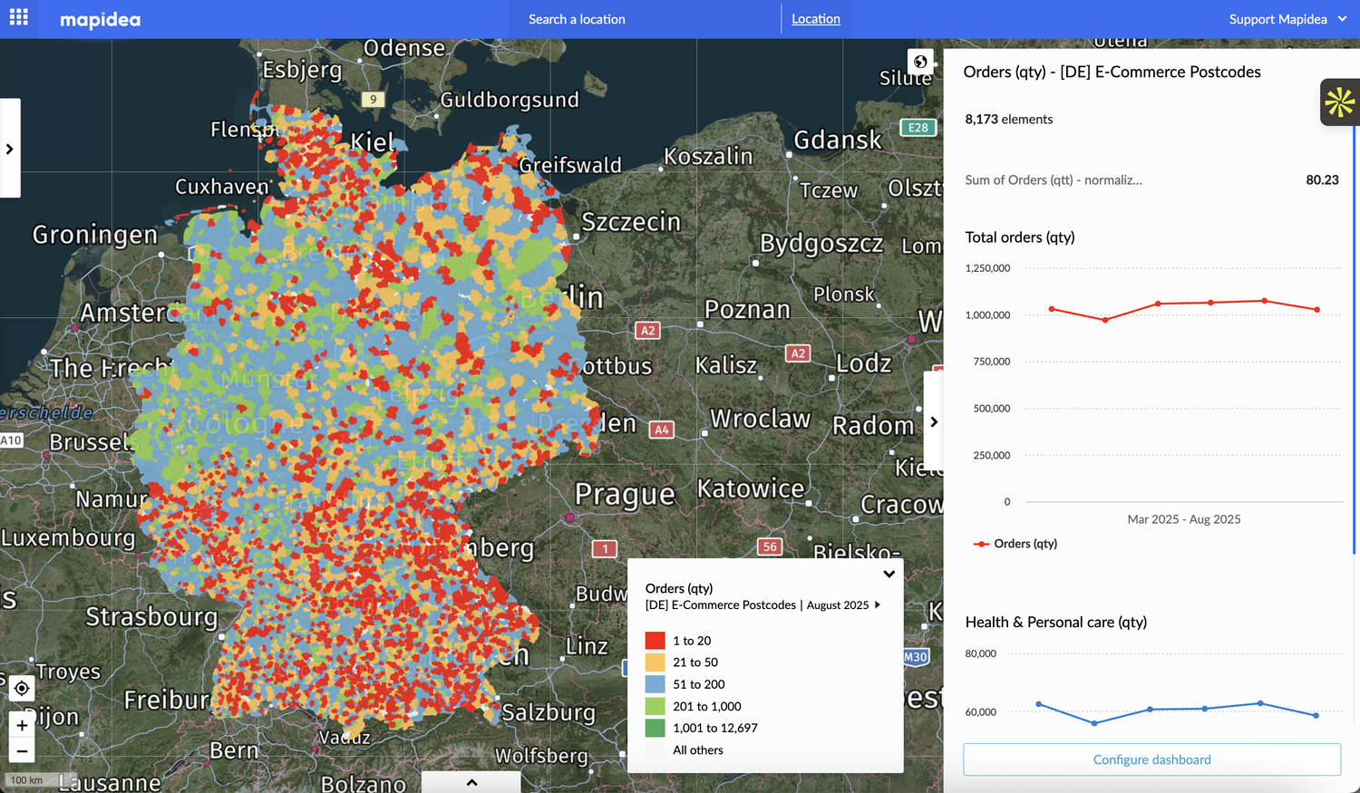

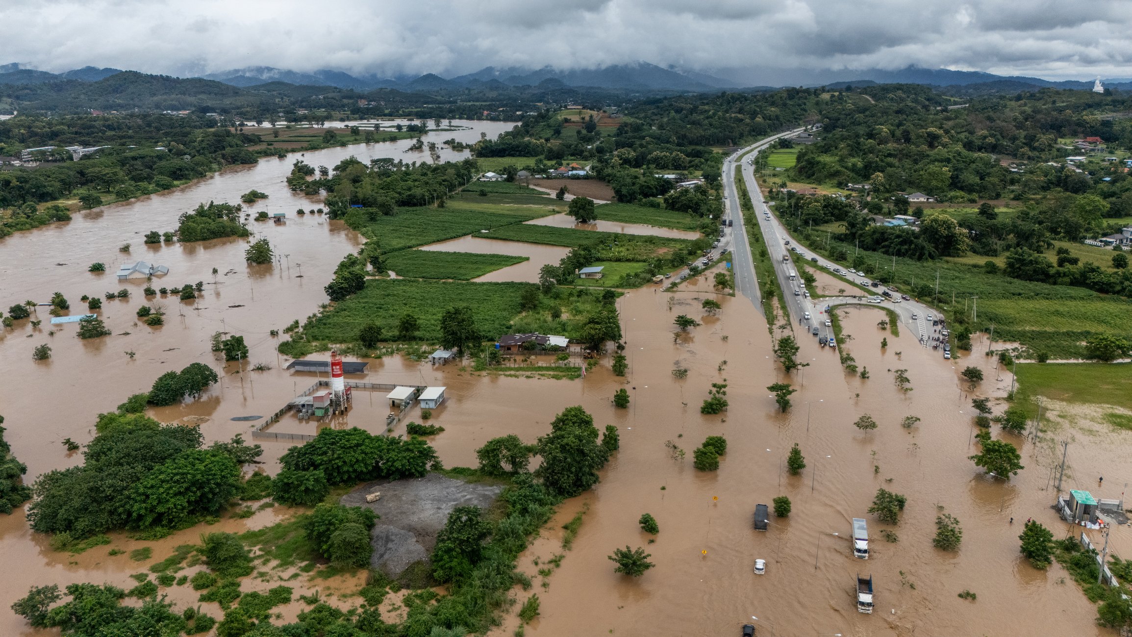
![Oslandia - (Fr) [Témoignage client] Jérôme STAUB, Colmar Agglomération](https://oslandia.com/wp-content/uploads/2025/11/t%C3%A9moignage-j%C3%A9rome-staub.png)
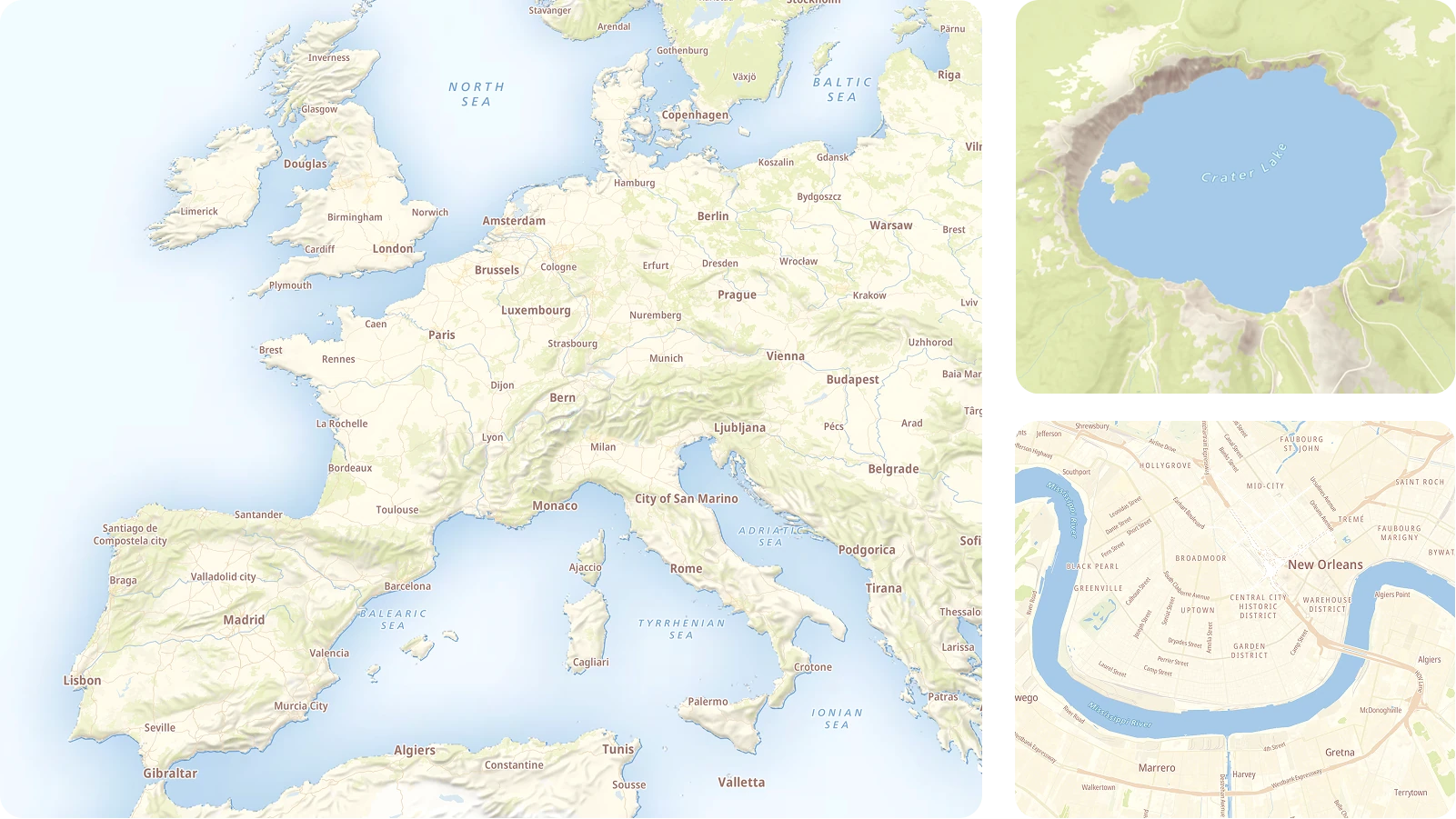


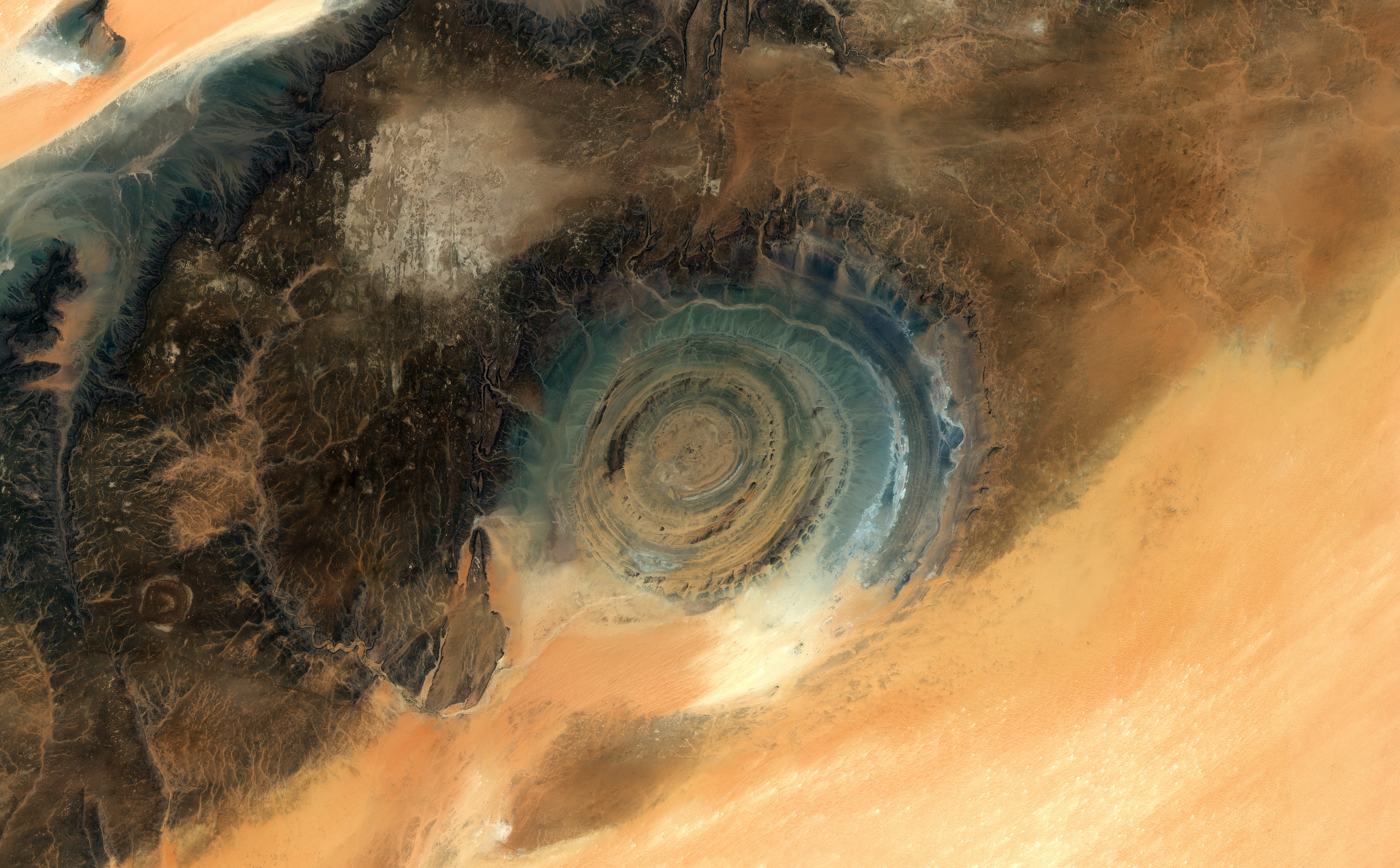

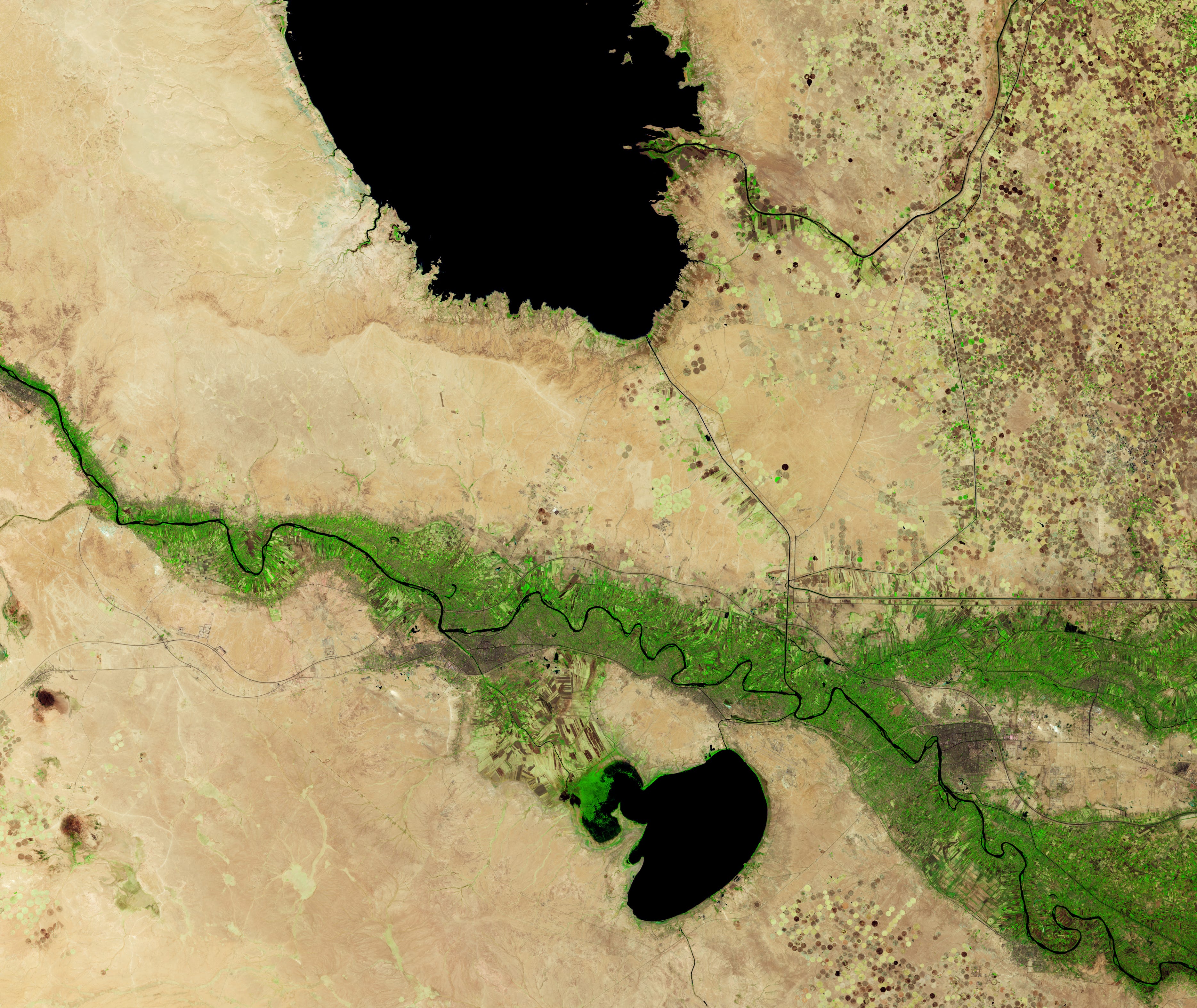

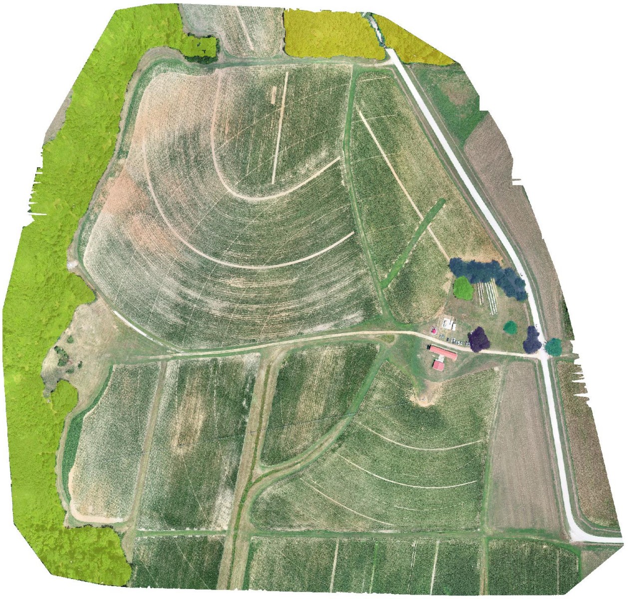
![Mergin Maps blog - [QGIS] How to collect GPS points for QGIS on Android with Mergin Maps](https://cdn.prod.website-files.com/64be358a4fb0e612b228bb9e/6936a50be2f9112e12fda97e_Image%207%20(2).jpg)
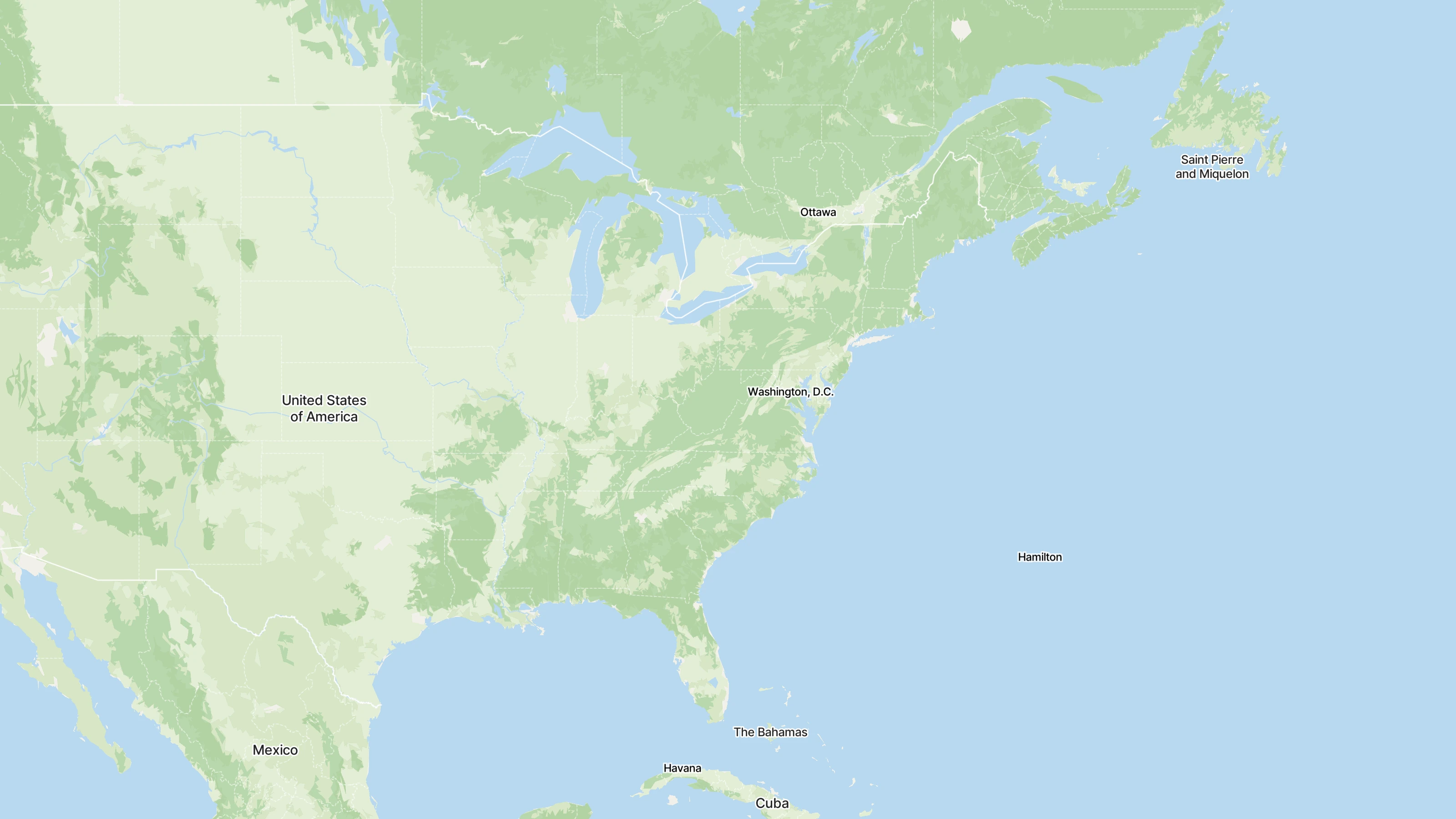


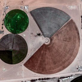


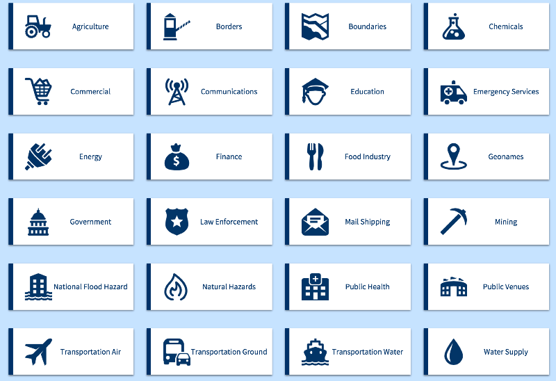
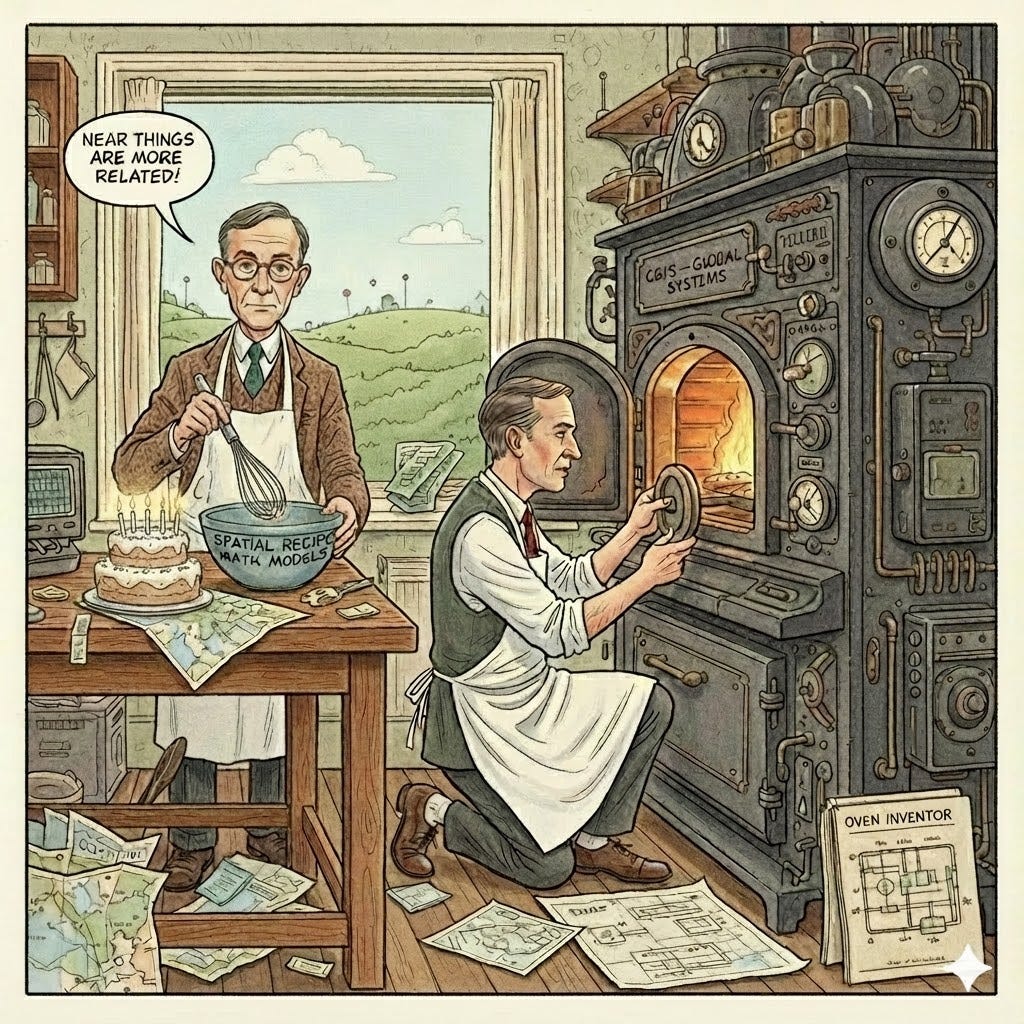
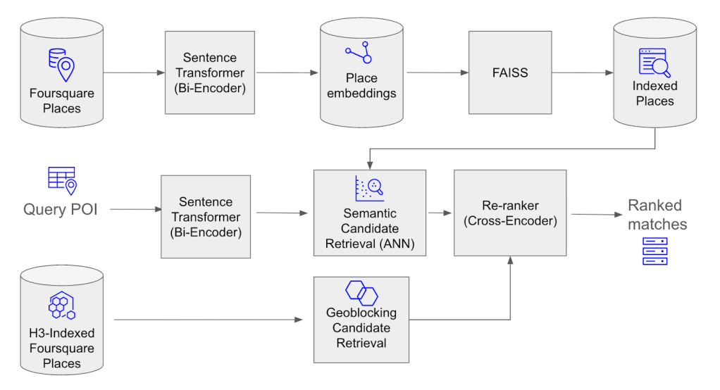


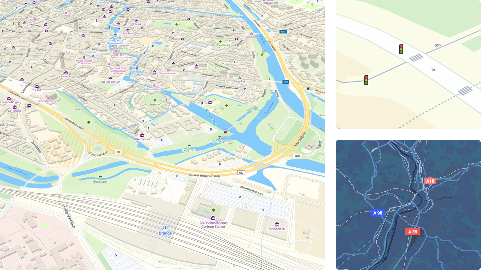

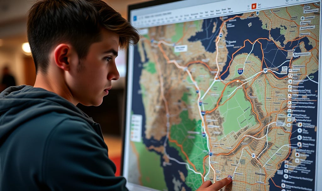

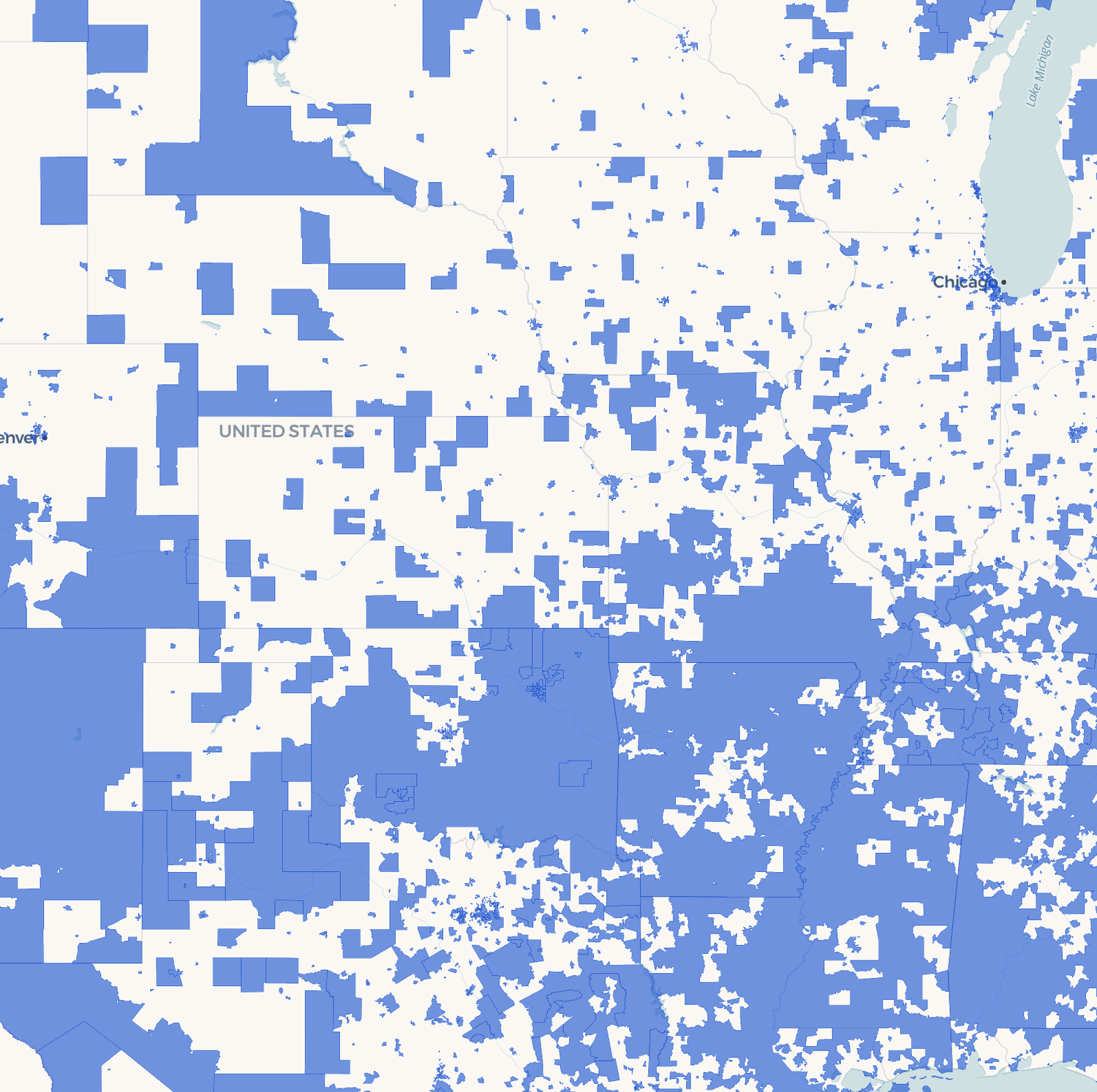


![Mergin Maps blog - [QGIS] How to use Mergin Maps to collaborate on QGIS projects](https://cdn.prod.website-files.com/64be358a4fb0e612b228bb9e/6672b4a9a58311472feb9f30_Image%2030.png)
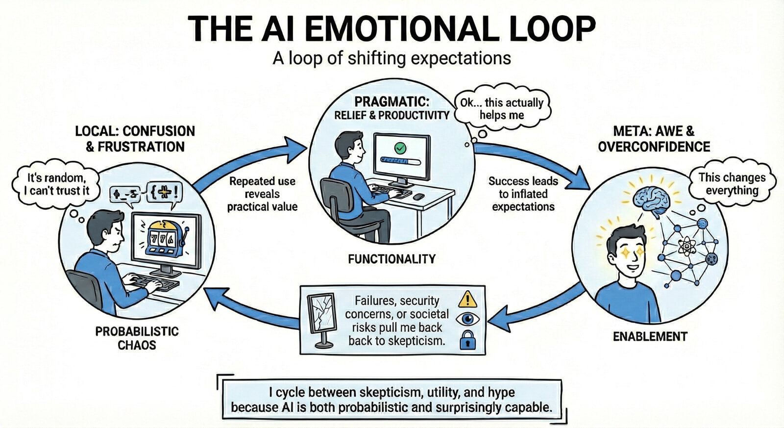


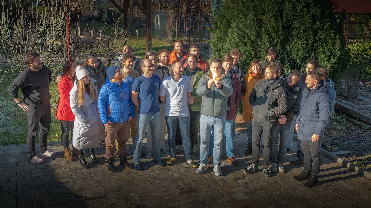

.png?format=1500w)

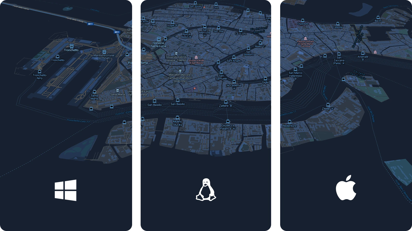


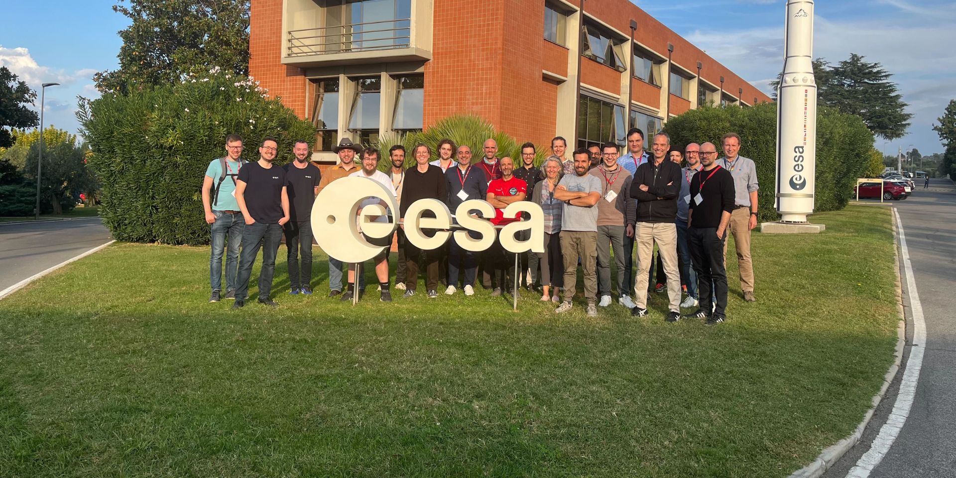


![Mergin Maps blog - [QGIS] Support Tip: Using HTML to improve your Mergin Maps project](https://cdn.prod.website-files.com/64be358a4fb0e612b228bb9e/691455af2c3e7ffea72bbef4_Image%2026%20(2).jpg)


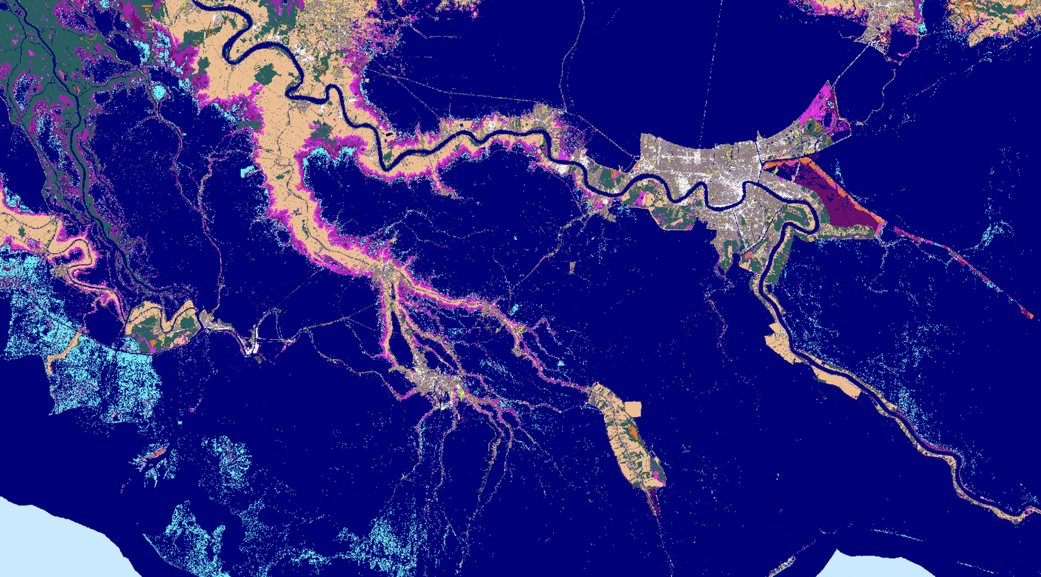


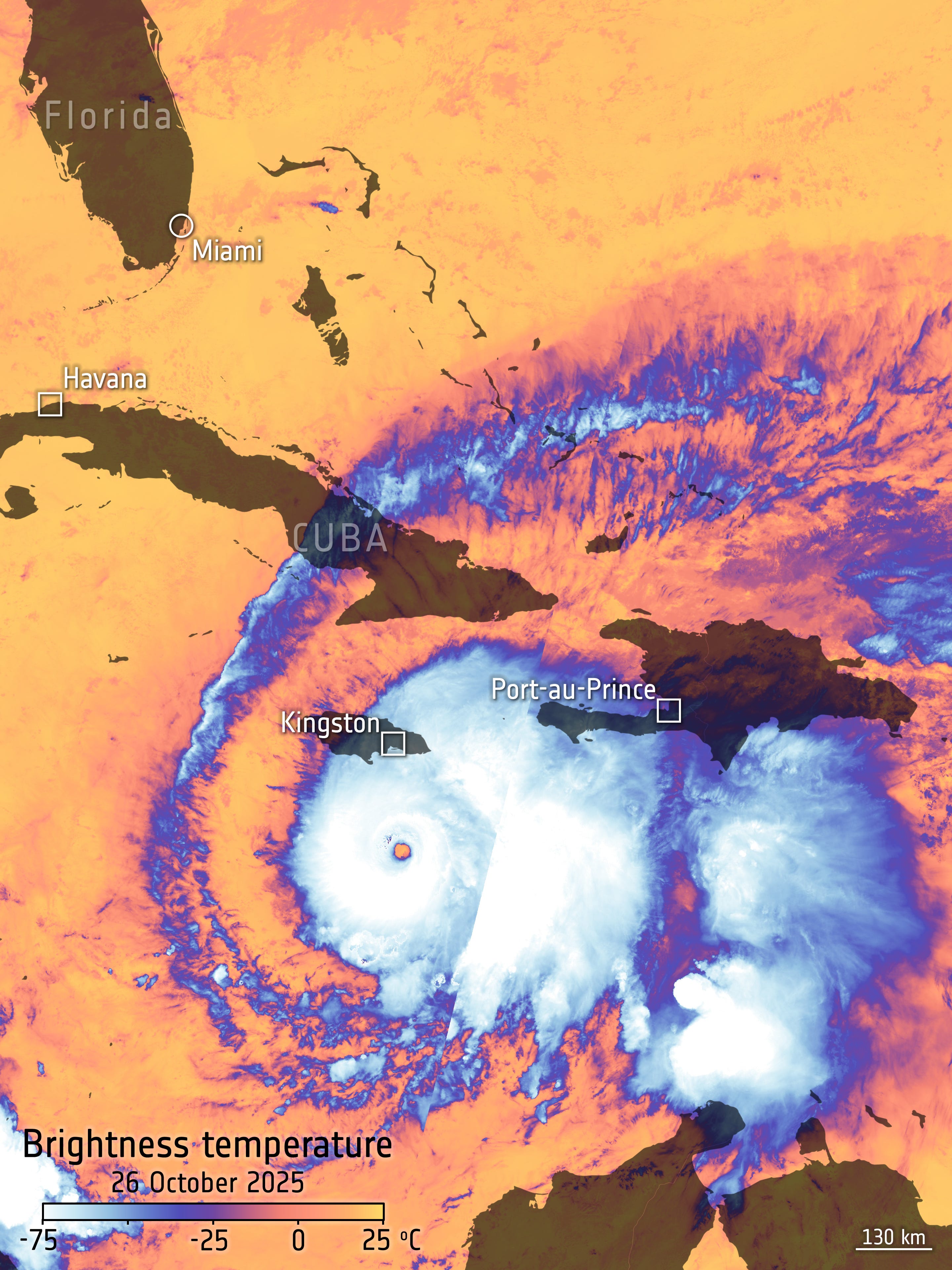


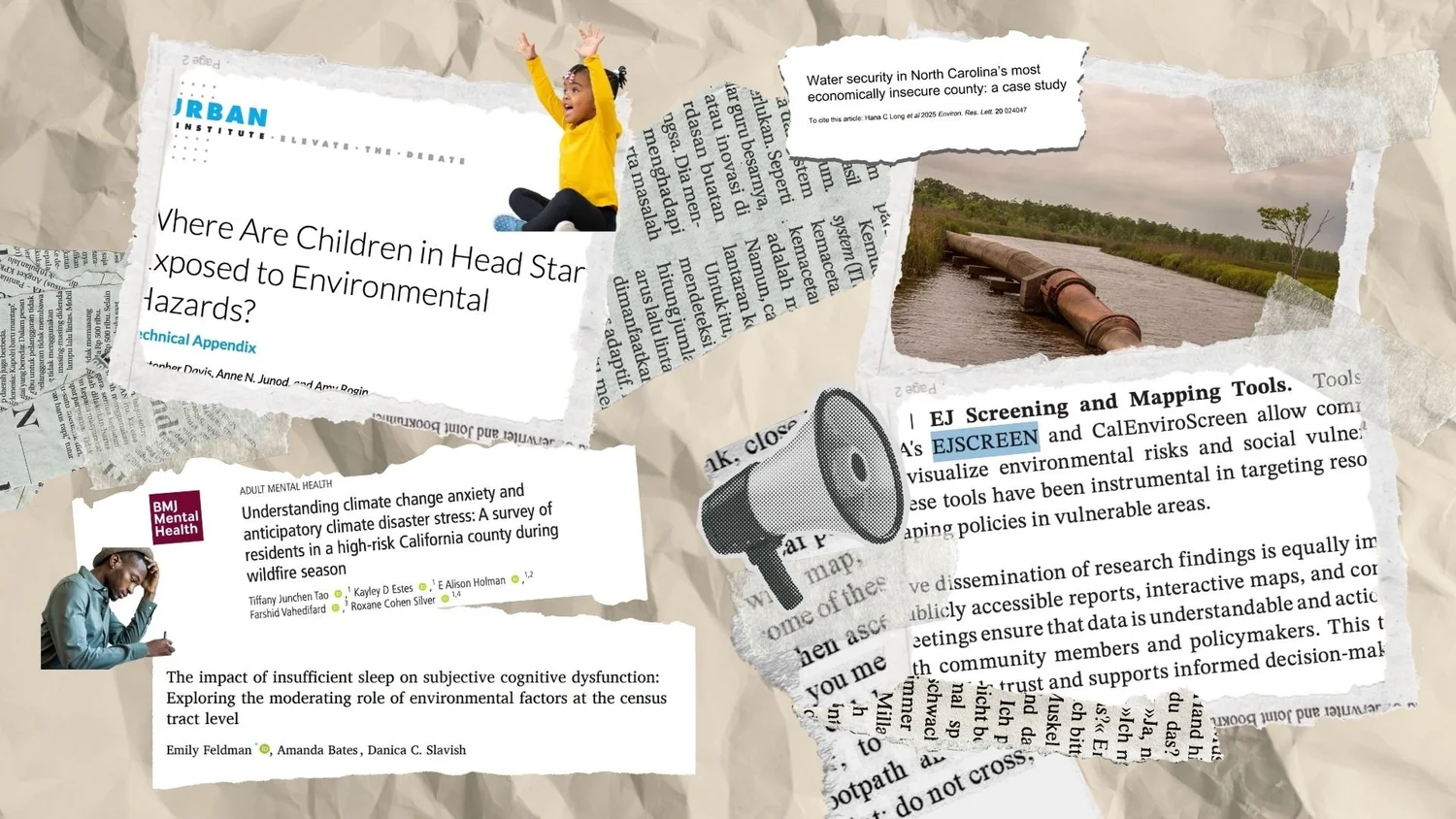

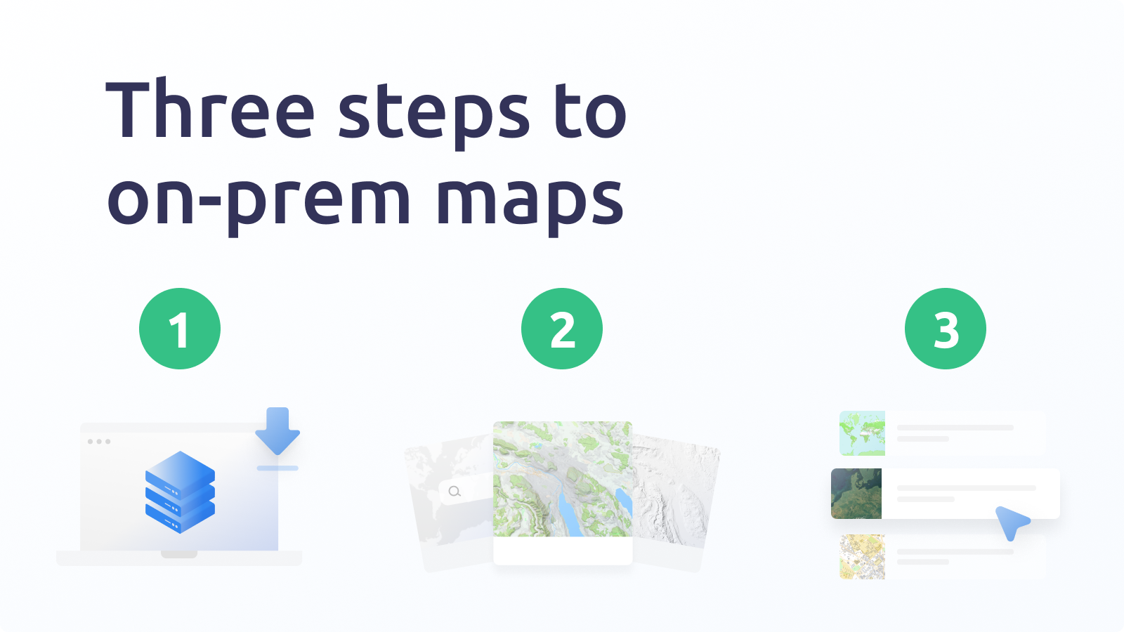

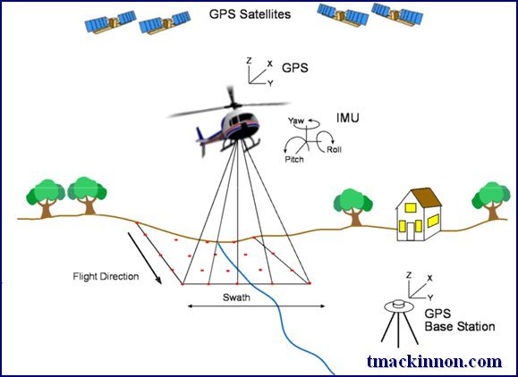
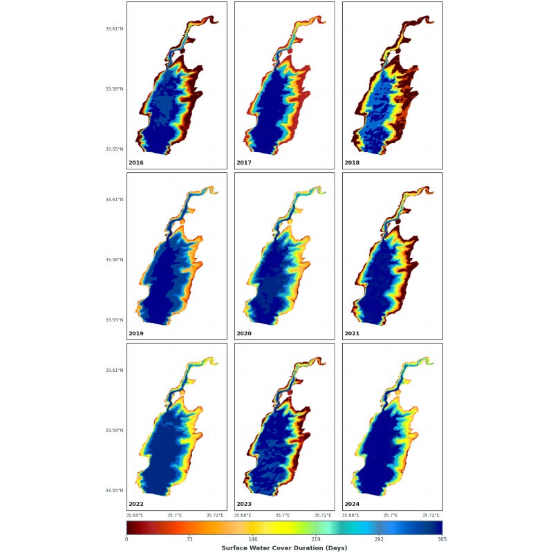
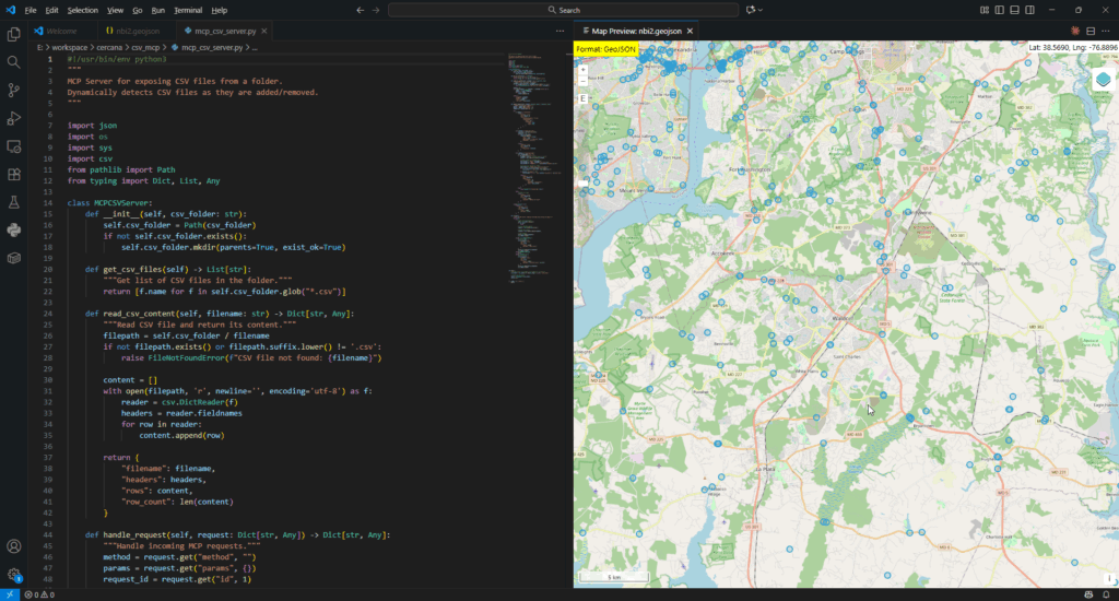


![Mergin Maps blog - [QGIS] Photo sketching is now available in Mergin Maps](https://cdn.prod.website-files.com/64be358a4fb0e612b228bb9e/6900db90d4a847f43551597d_Image%2027%20(2).jpg)


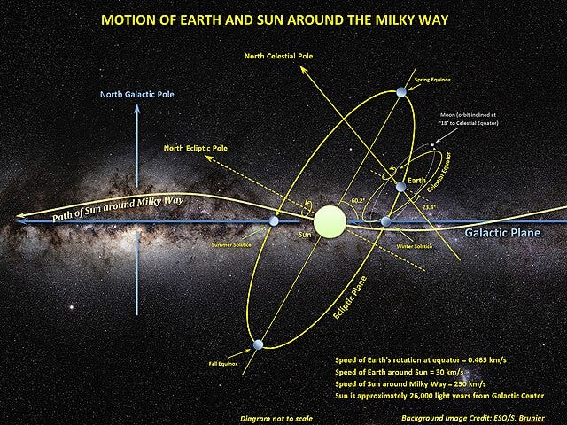


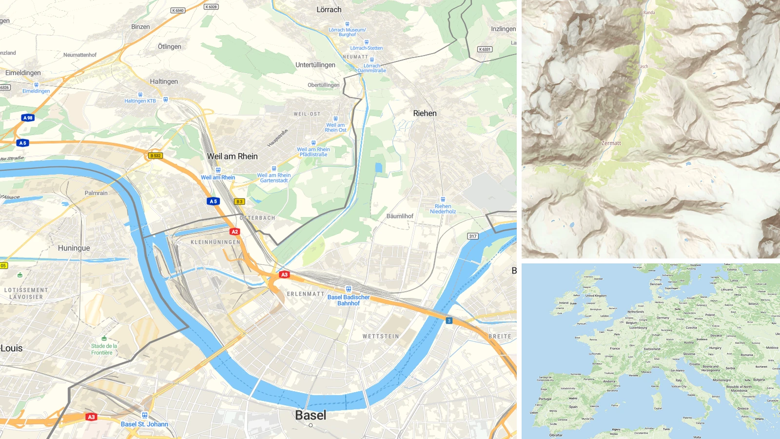
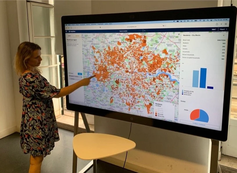
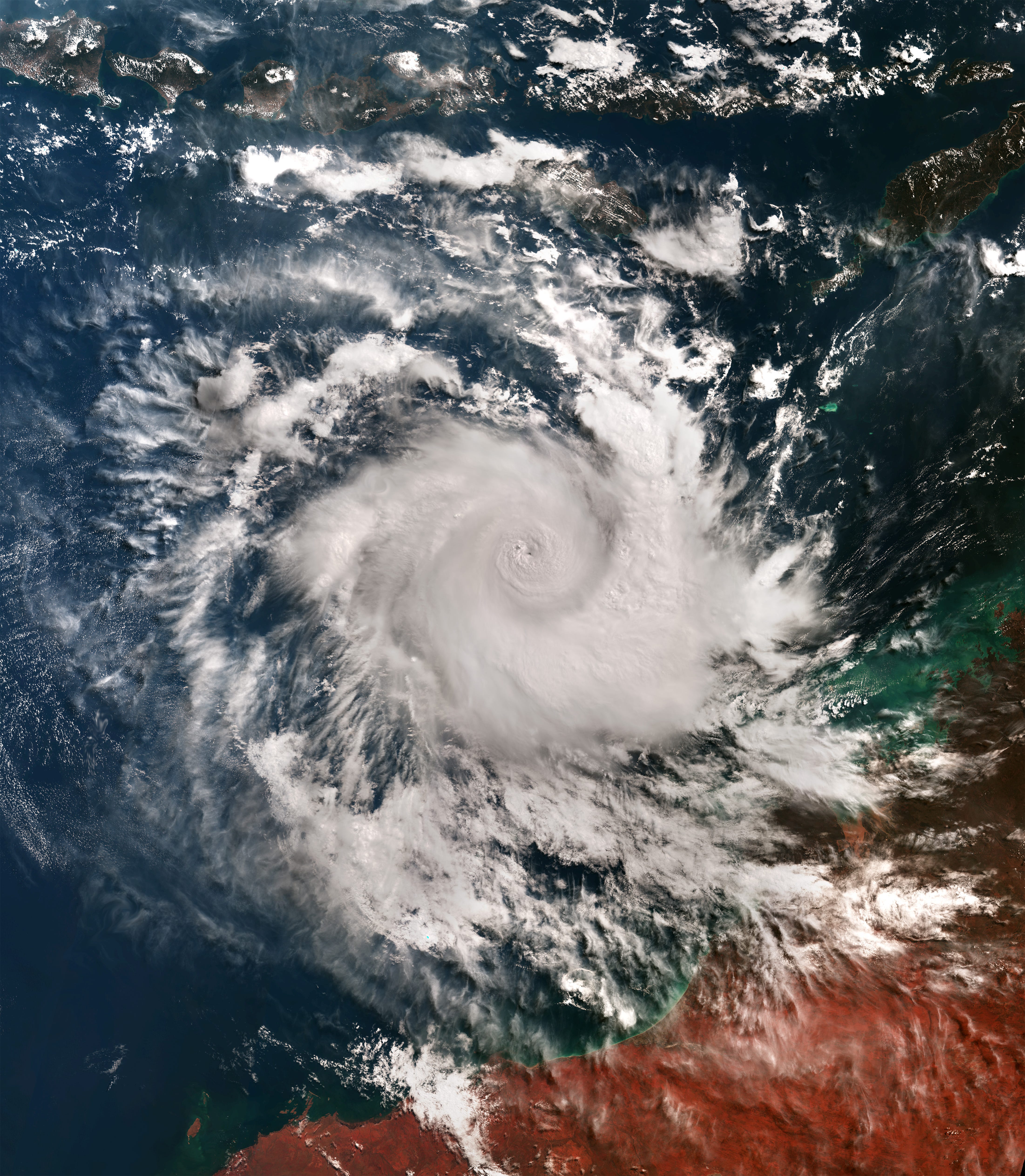
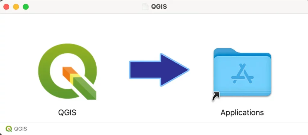


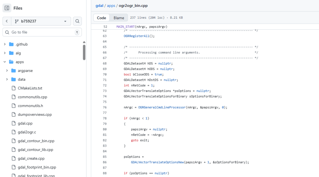

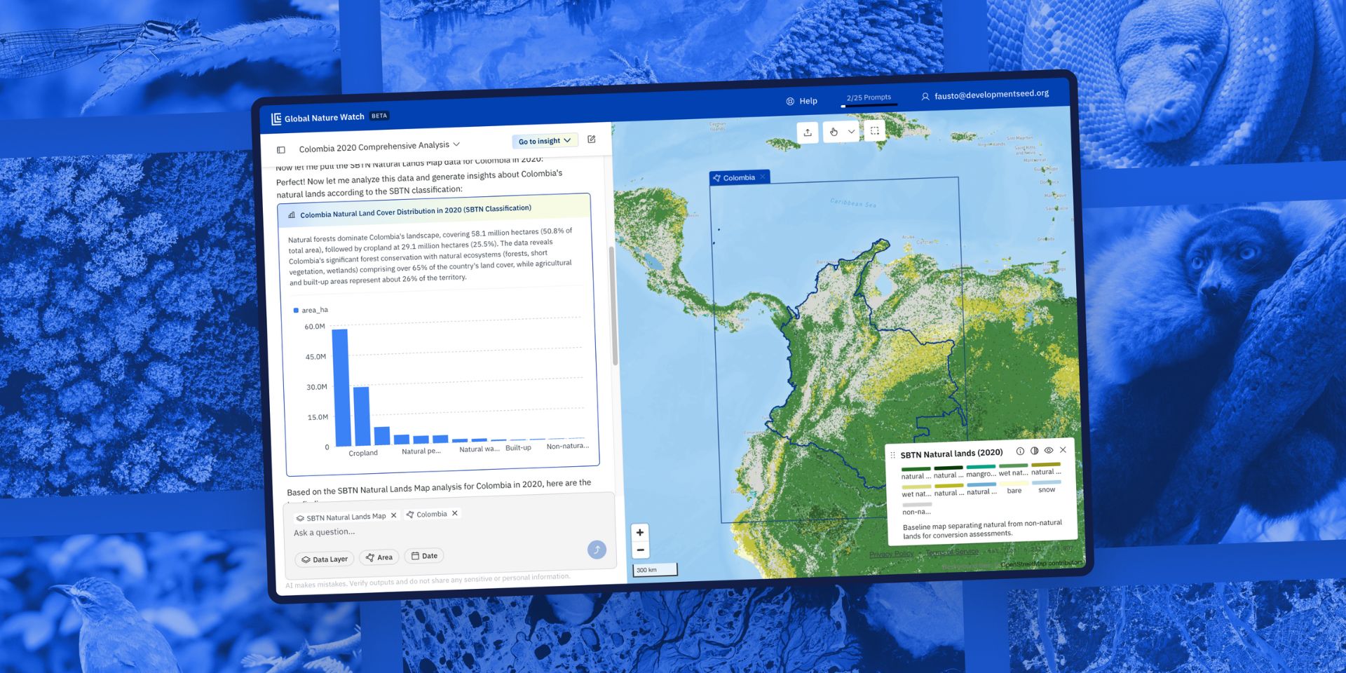
.jpg?format=1500w)


![Mergin Maps blog - [QGIS] Best practices for user management in Mergin Maps](https://cdn.prod.website-files.com/64be358a4fb0e612b228bb9e/68e8c650a265f48562c85d8e_Image%2024%20(1).jpg)


![Mergin Maps case studies - [QGIS] Ensuring regulatory compliance for water distribution in Portugal](https://cdn.prod.website-files.com/64be358a4fb0e612b228bb9e/68e7d3d5ea49a6d23403bc35_488205375_1274711351107216_5408279484773325065_nCUT2.jpg)


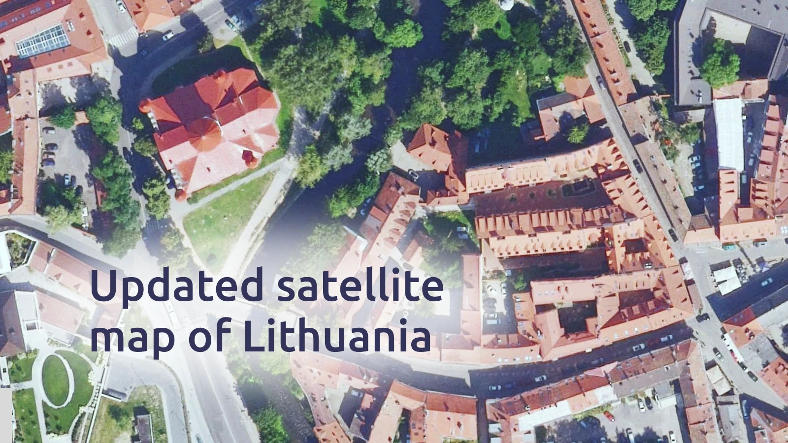
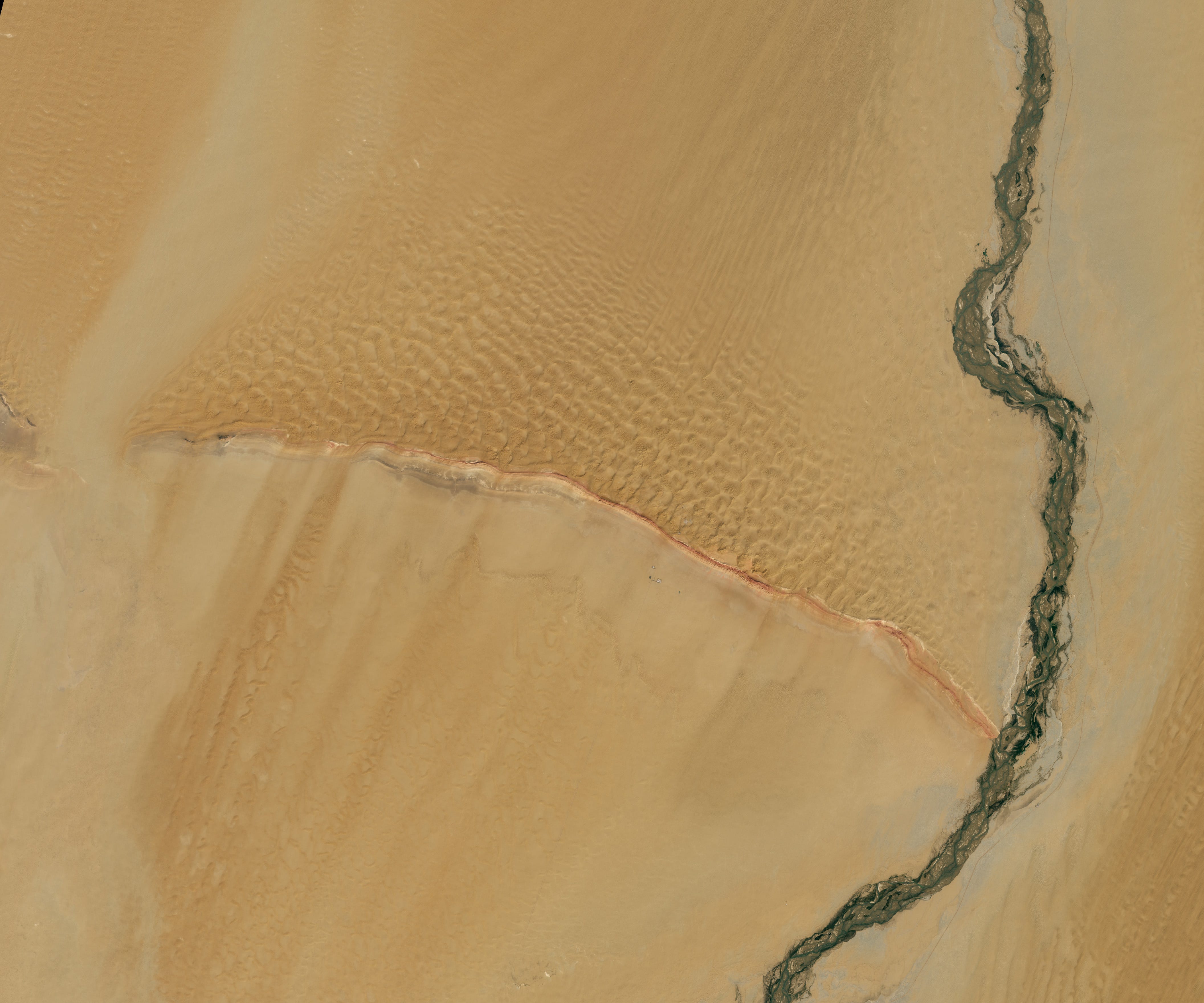
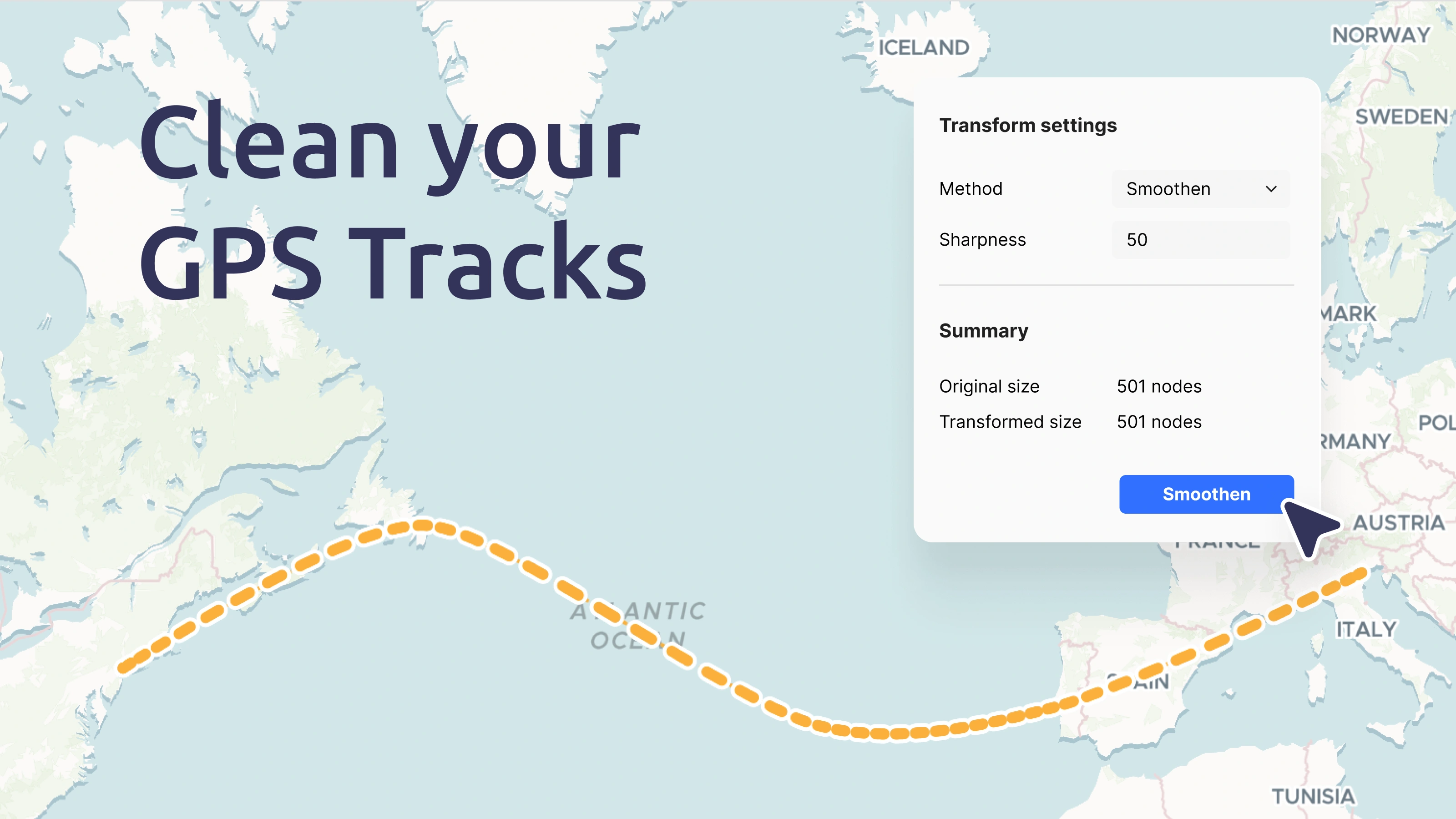
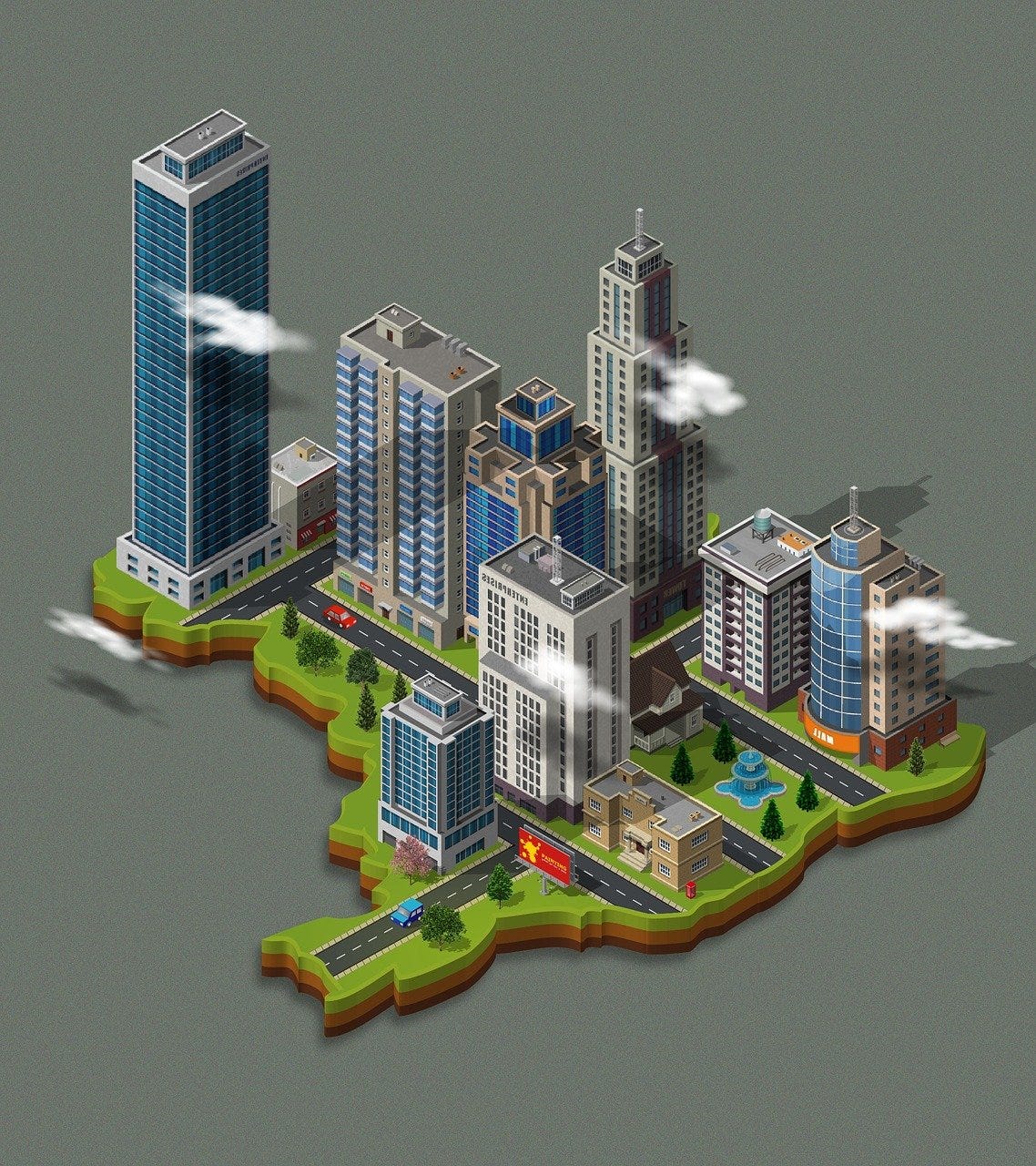

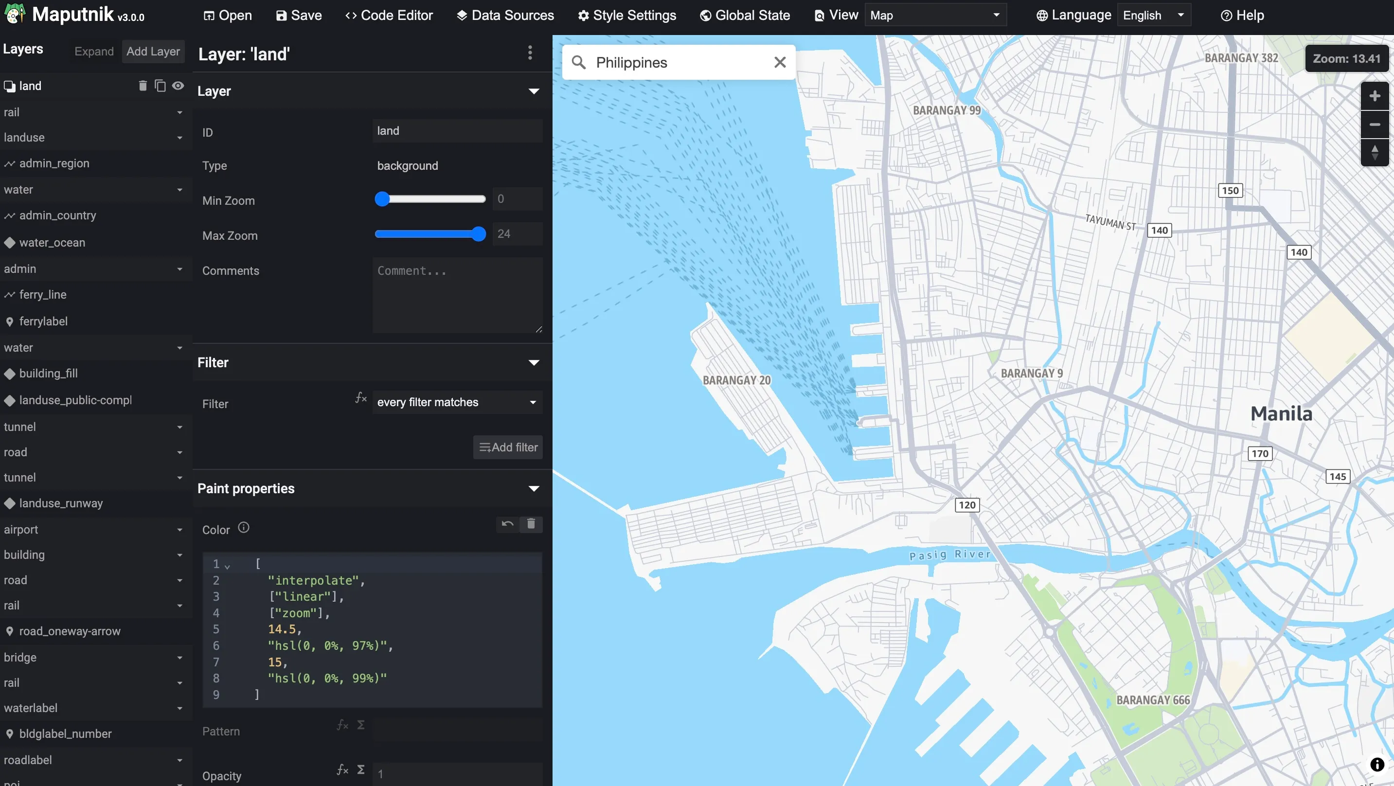

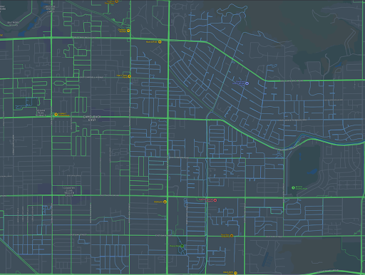
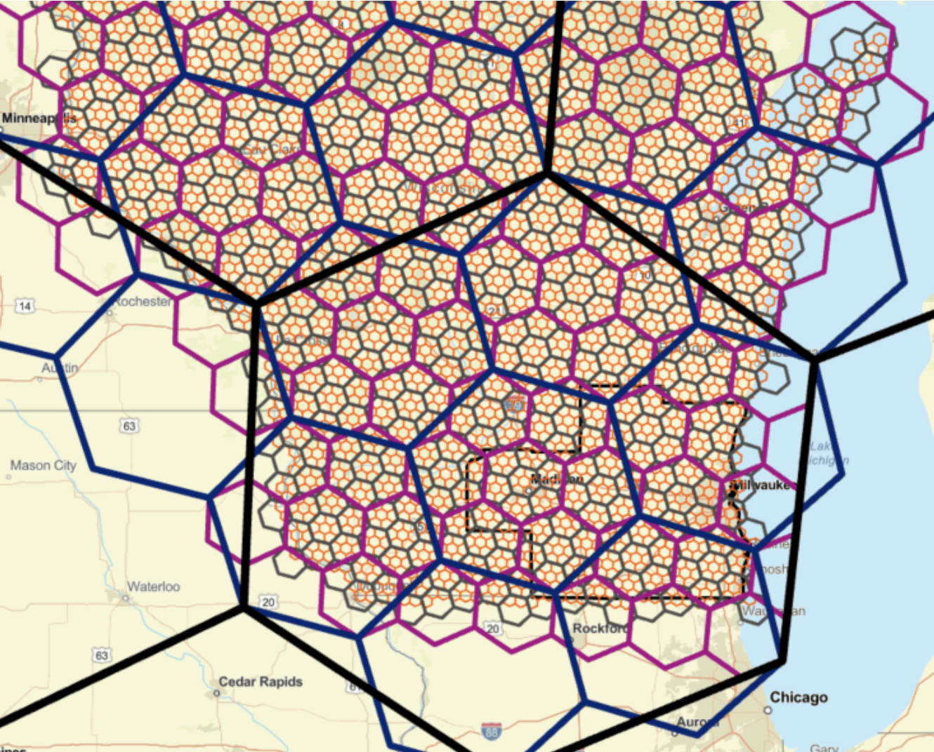

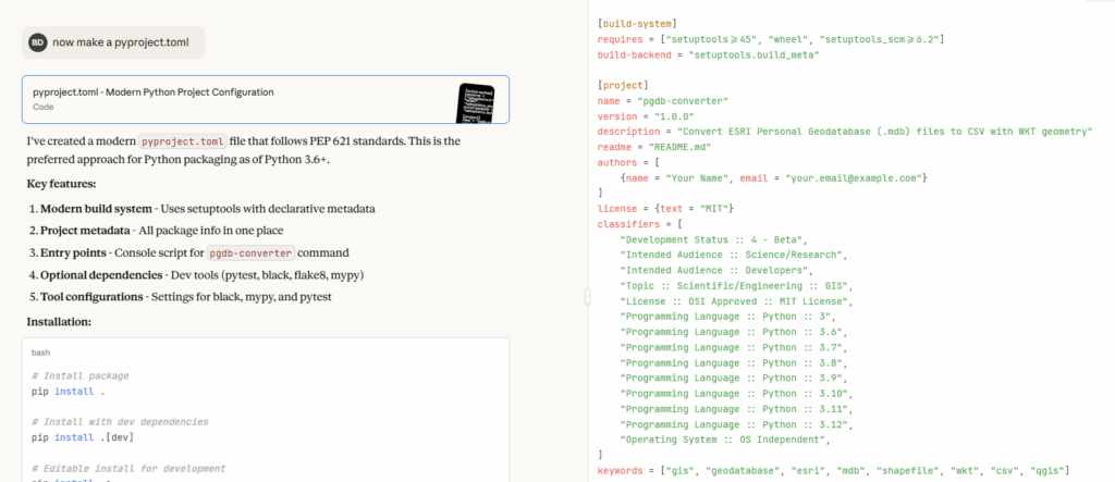
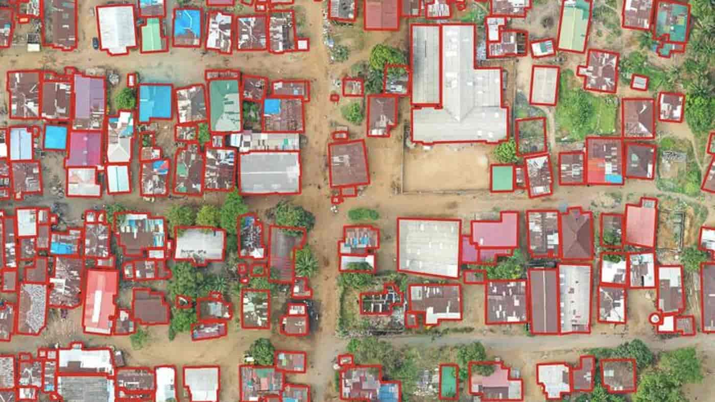
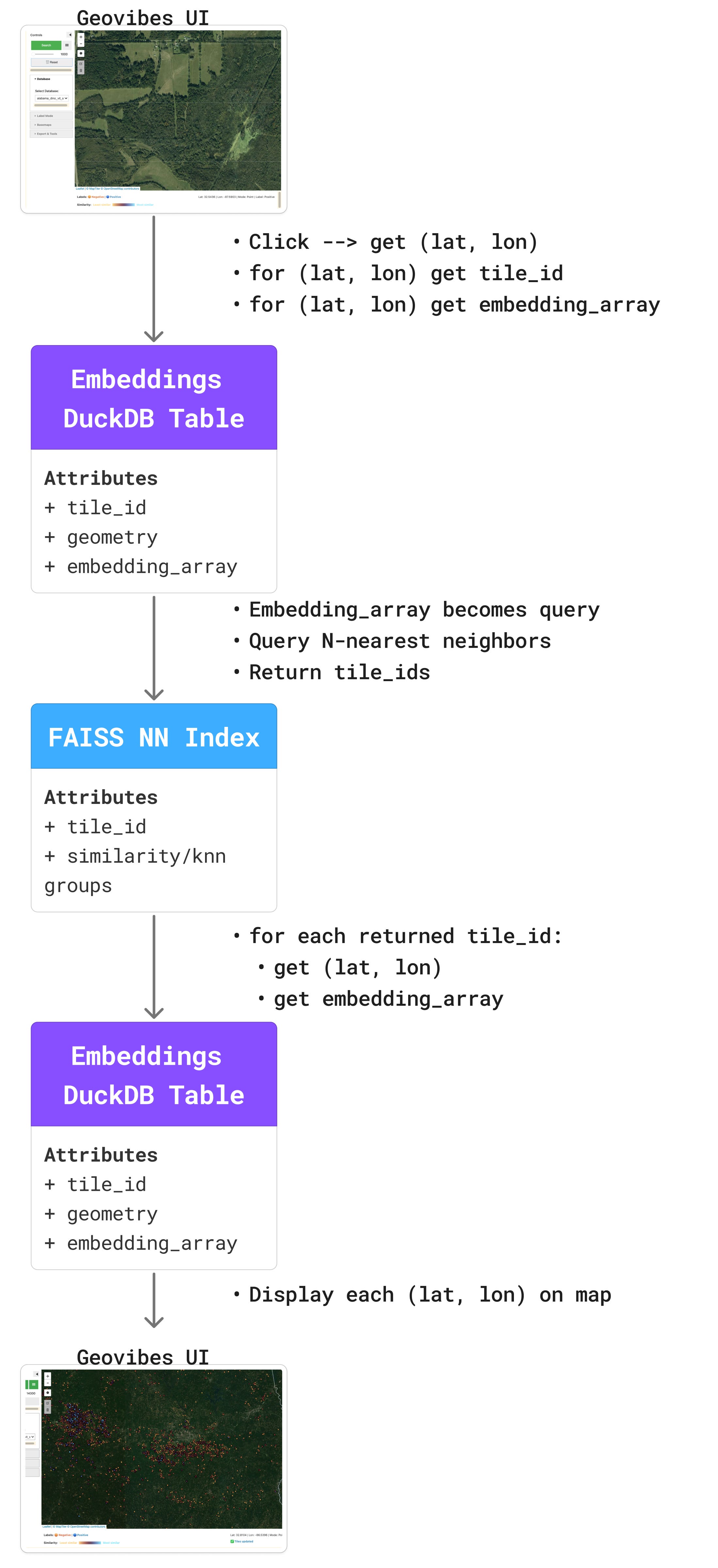


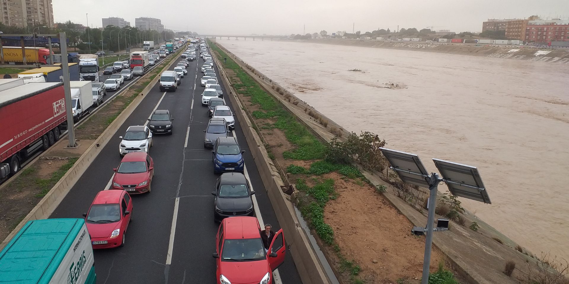


![Mergin Maps case studies - [QGIS] Involving communities in conservation through citizen science](https://cdn.prod.website-files.com/64be358a4fb0e612b228bb9e/68d3a1d9675b41c874e1d7d3_Copy%20of%200043_ojoaocruz_VERDE_GVEDP_Sabugal_20250406_cut.jpg)


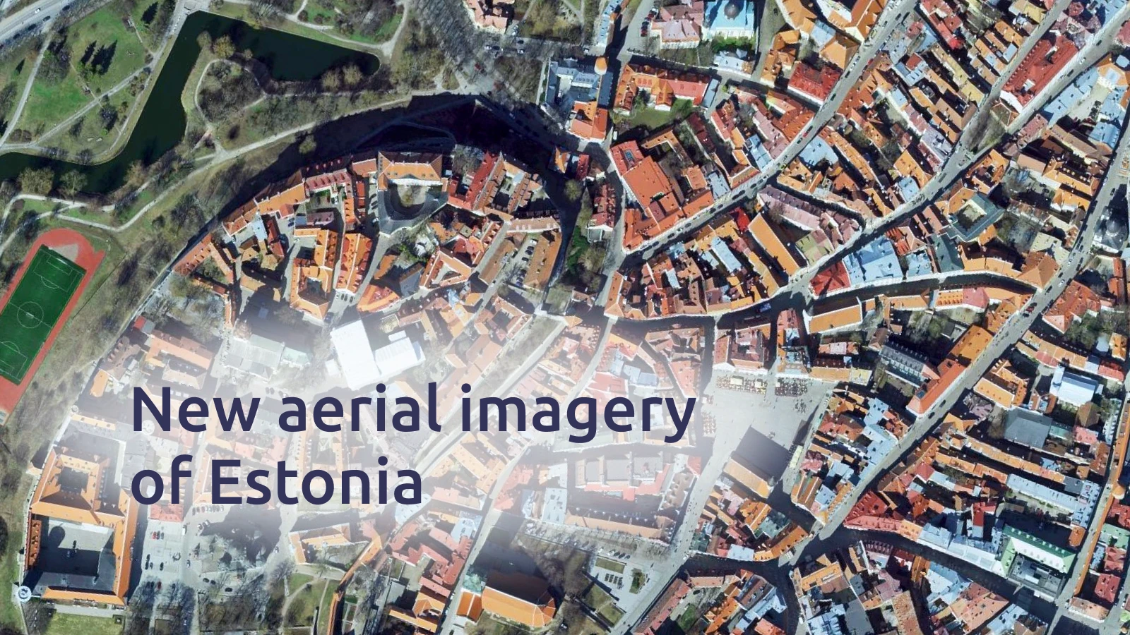

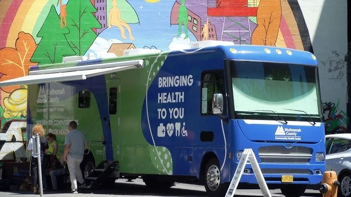
![Mergin Maps blog - [QGIS] Create professional survey reports using QGIS Print Layout after field data collection](https://cdn.prod.website-files.com/64be358a4fb0e612b228bb9e/68c8271ac4390348acdaf45f_blog_main.png)

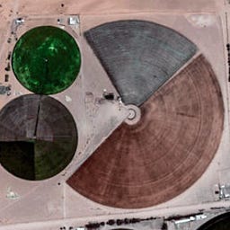


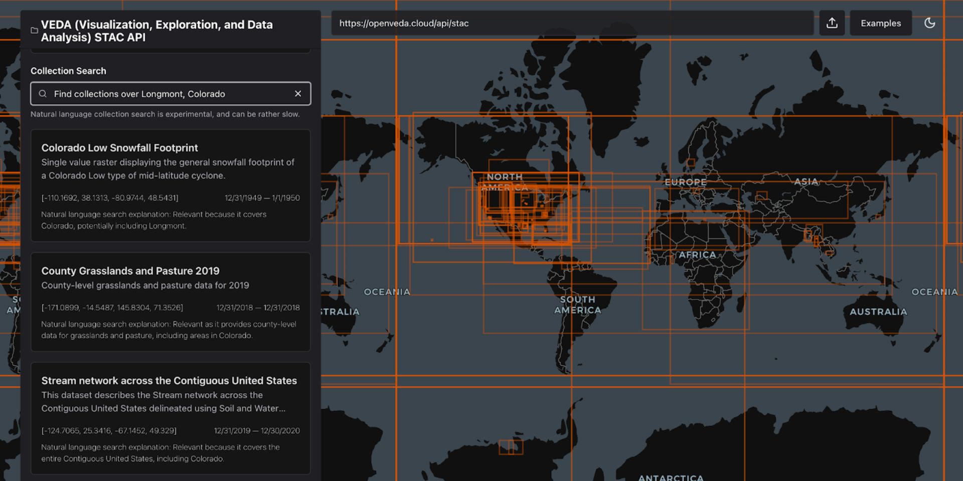


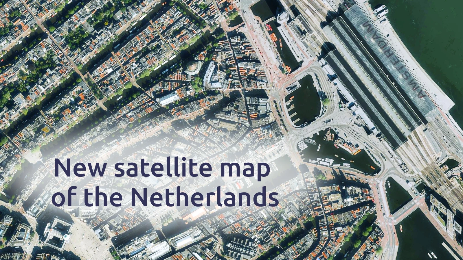
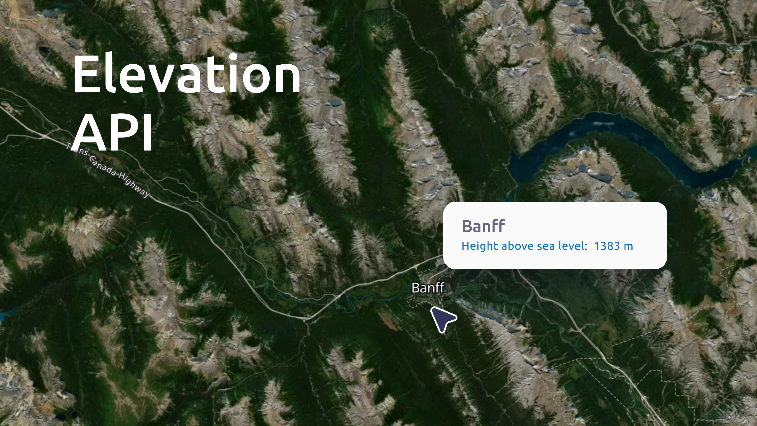


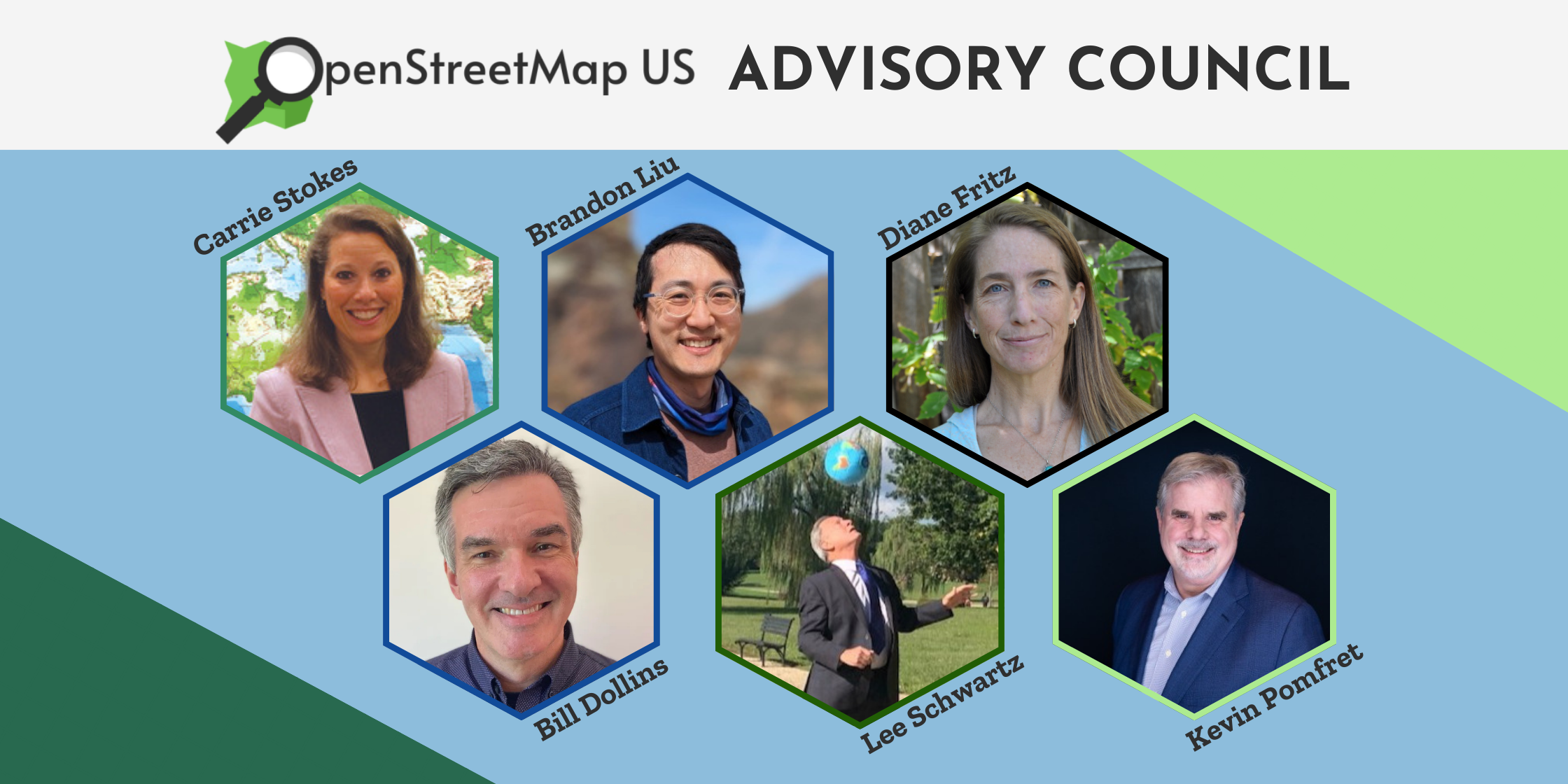
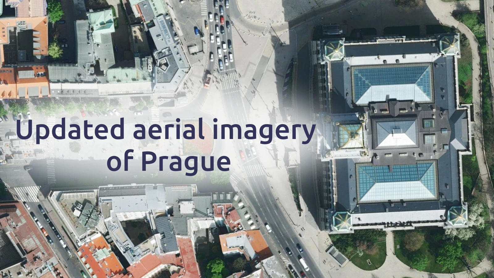


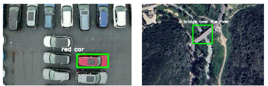


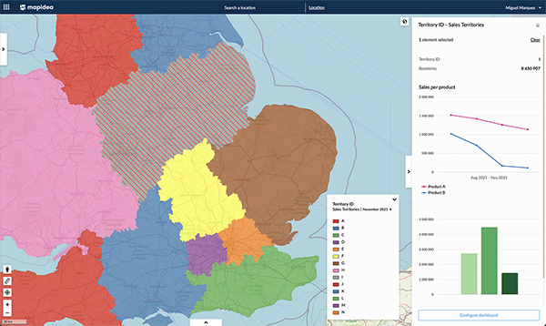
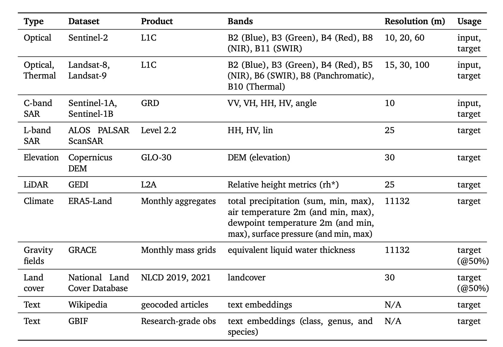

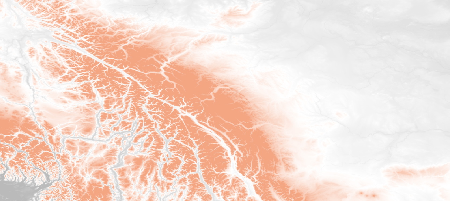
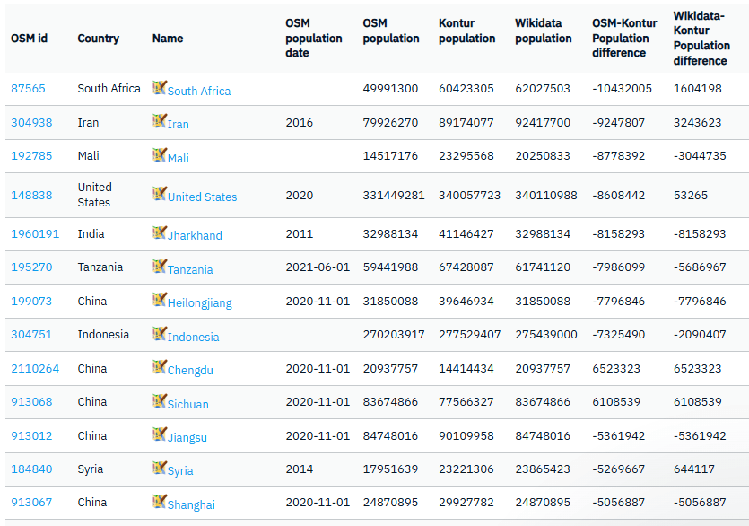


![Mergin Maps case studies - [QGIS] Monitoring historic buildings in Derbyshire](https://cdn.prod.website-files.com/64be358a4fb0e612b228bb9e/68933c2682db0eeabce2d60e_The%20Grade%20II%20listed%20Derby%20Silk%20Mill%2C%20now%20the%20Museum%20of%20Making_cutout.jpg)


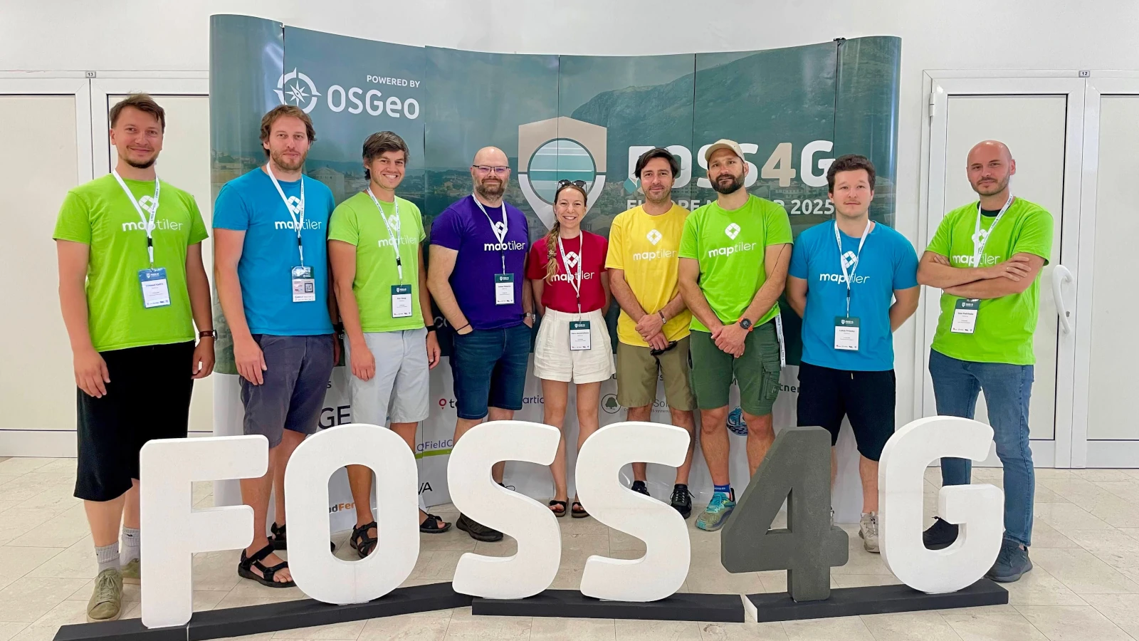
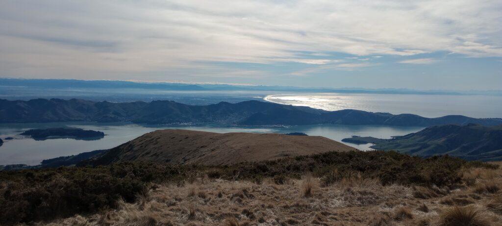
![Mergin Maps blog - [QGIS] Mergin Maps gets sketchy](https://cdn.prod.website-files.com/64be358a4fb0e612b228bb9e/688b3145bedd990f90bc431c_Map%20Sketching%20(2).jpg)
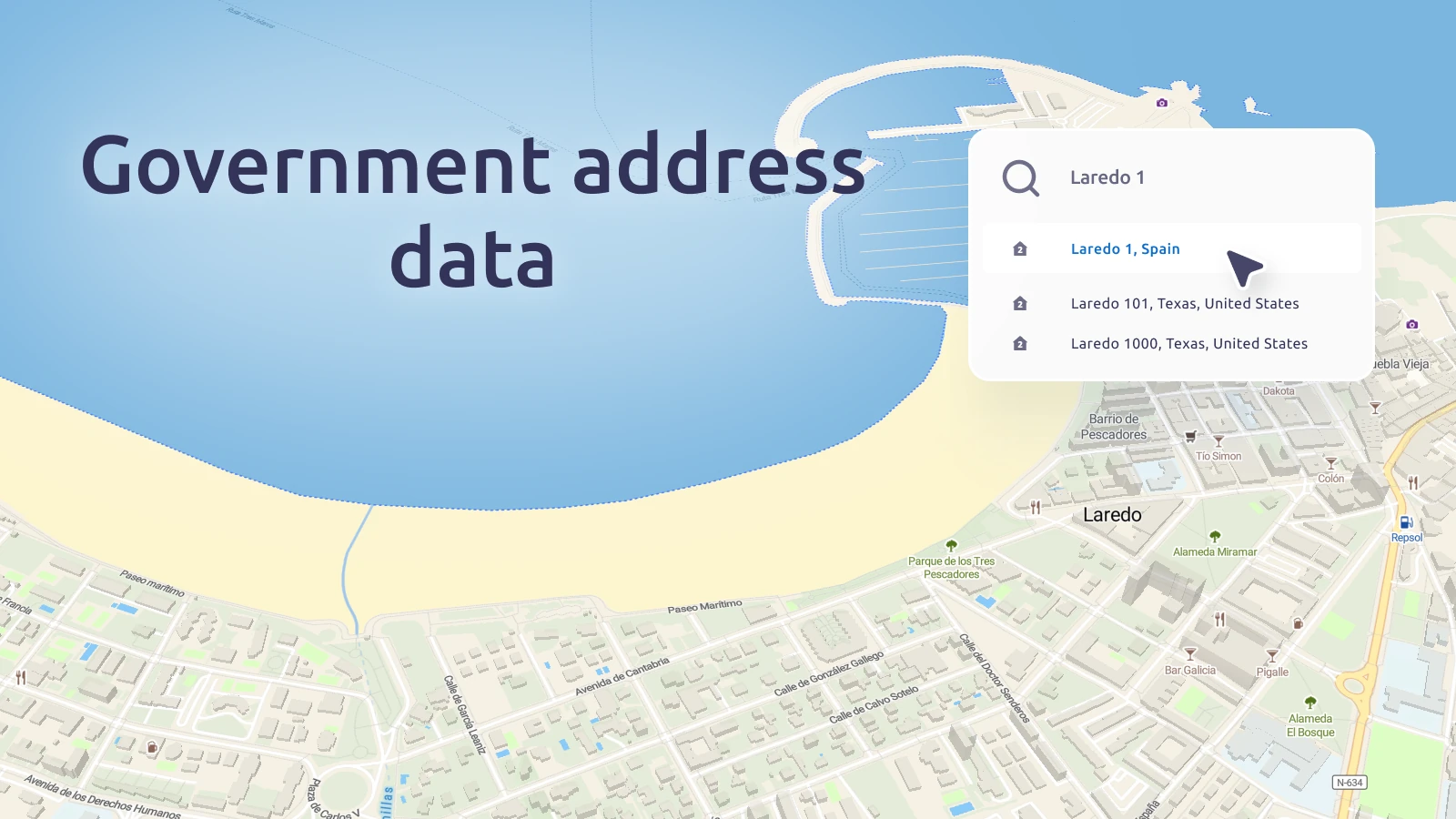
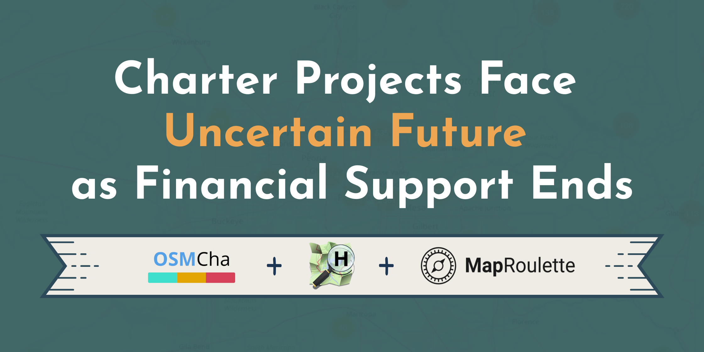


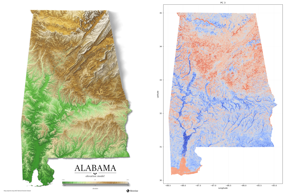
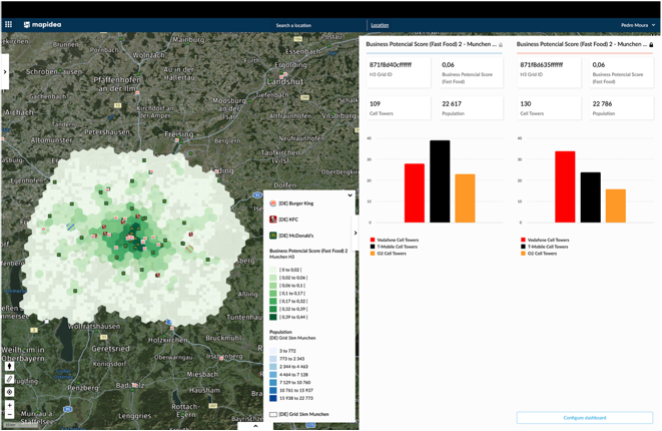
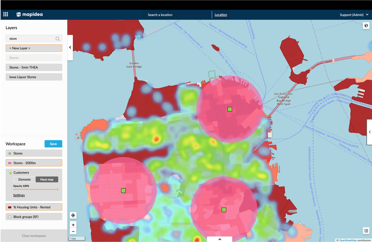
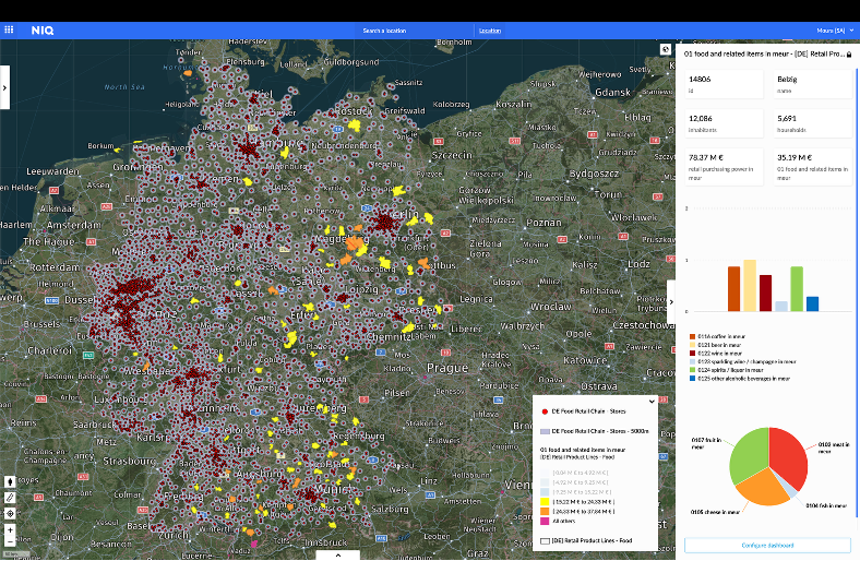

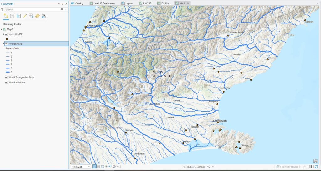


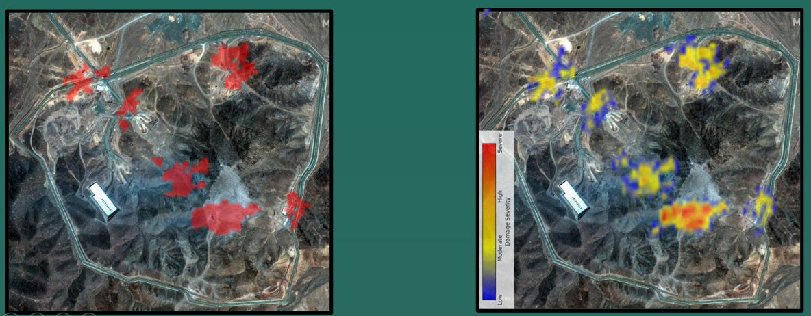


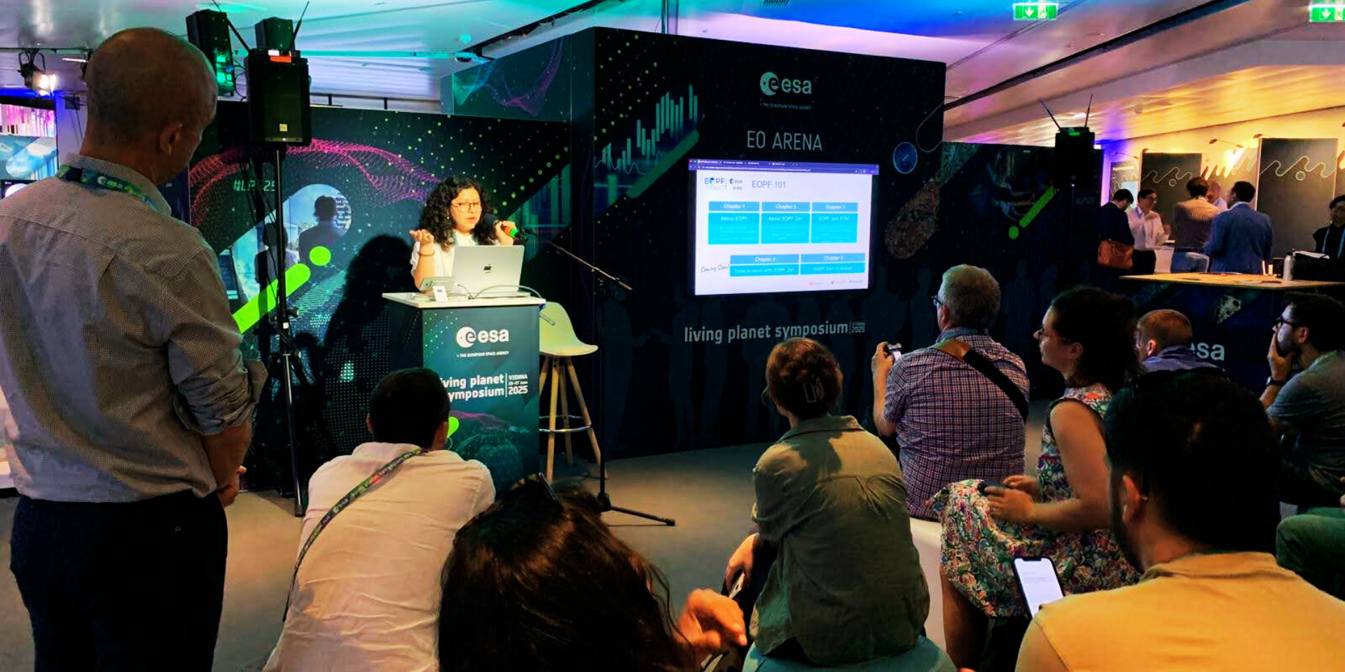
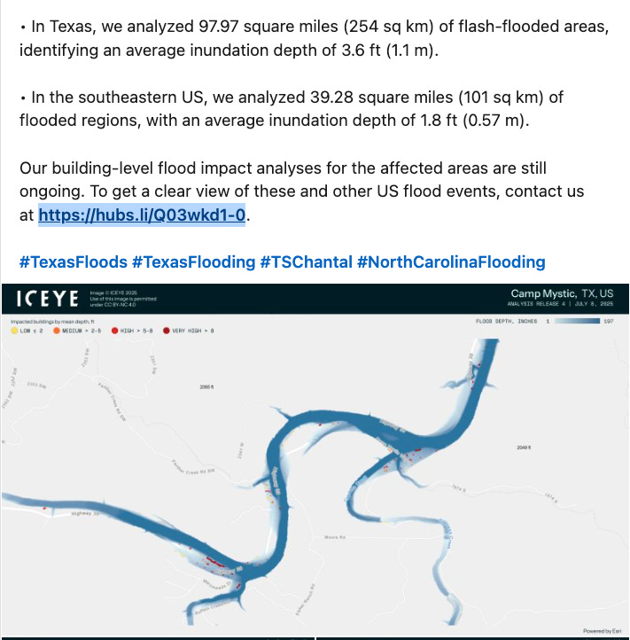
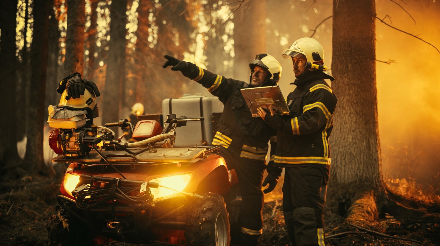


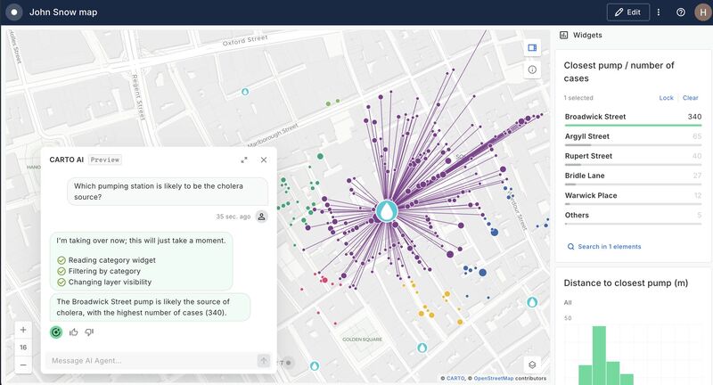

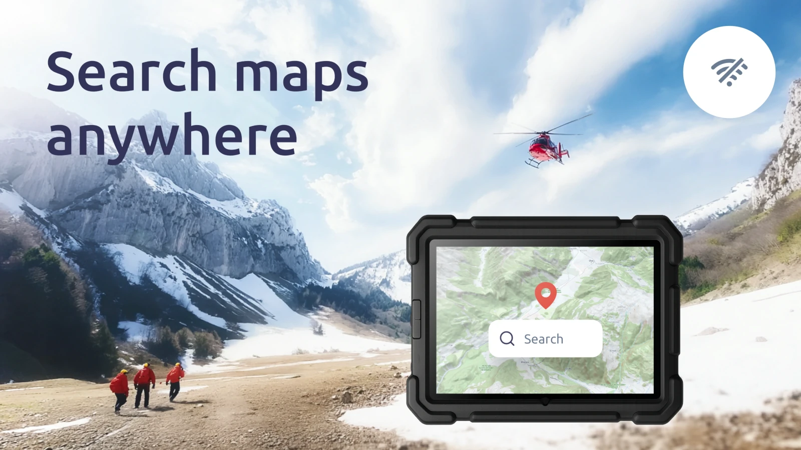


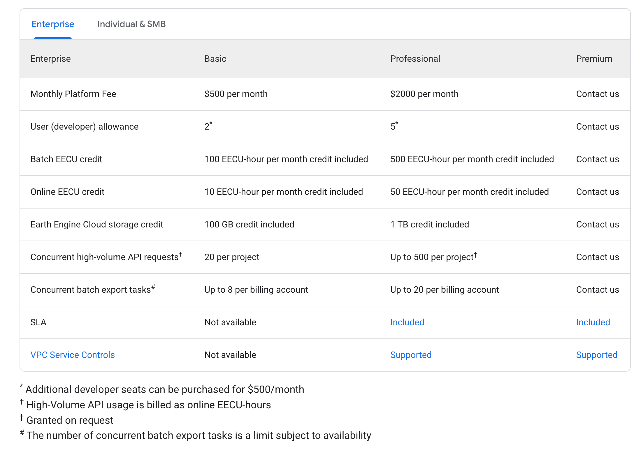


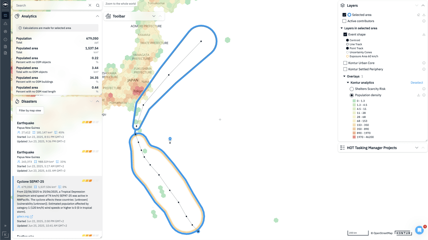

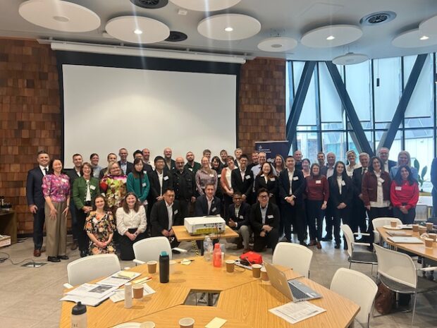


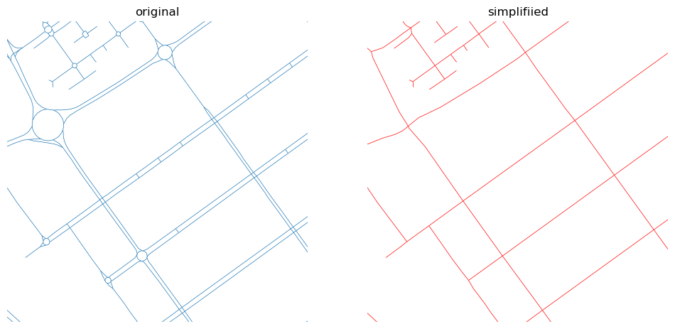


.jpg)


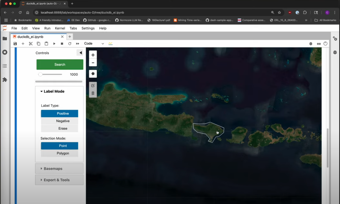
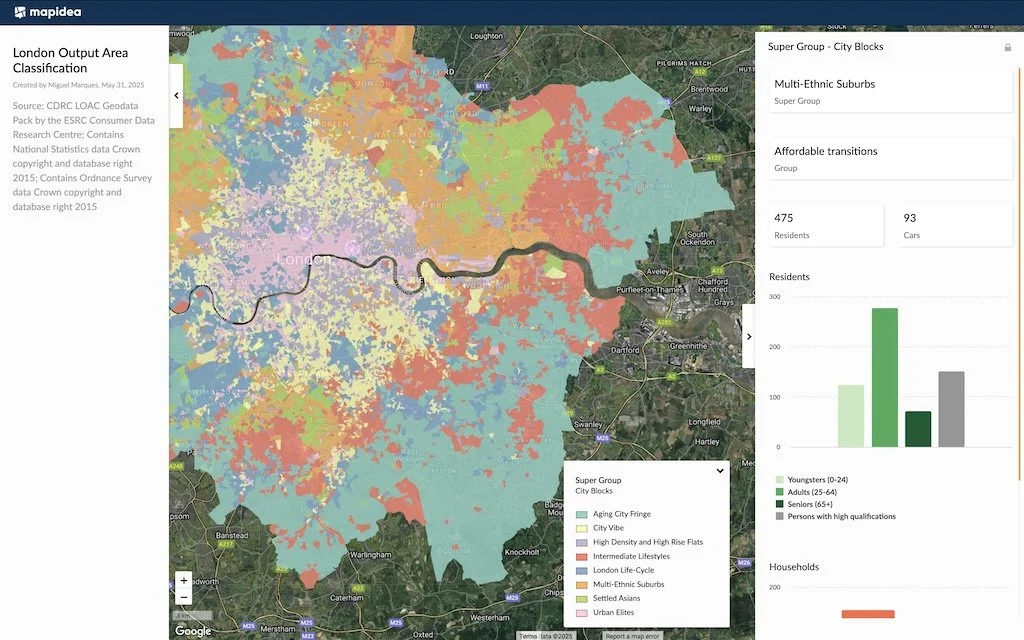


![Mergin Maps blog - [QGIS] New API tools give you more user management options!](https://cdn.prod.website-files.com/64be358a4fb0e612b228bb9e/683961345ceb5bb40c373cc4_Image%2028.jpg)


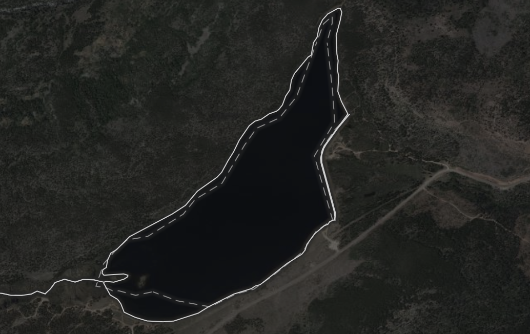

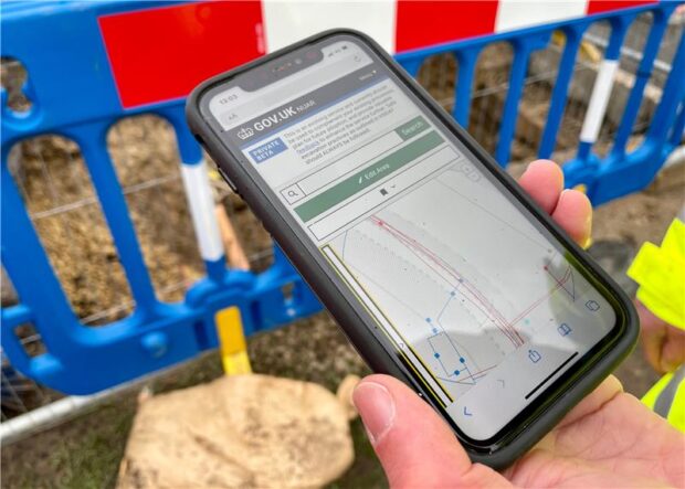

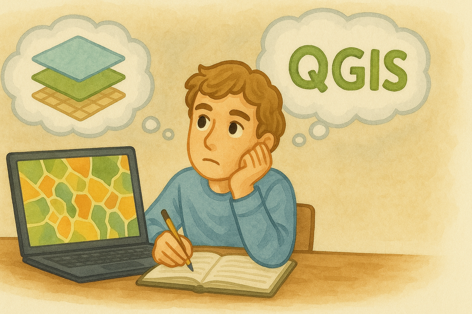

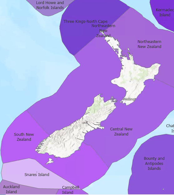
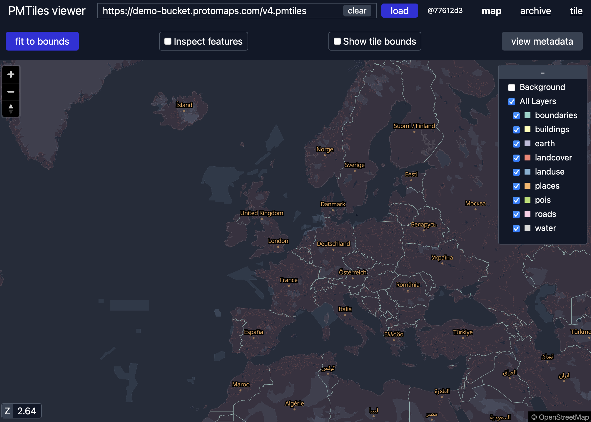
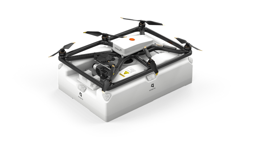


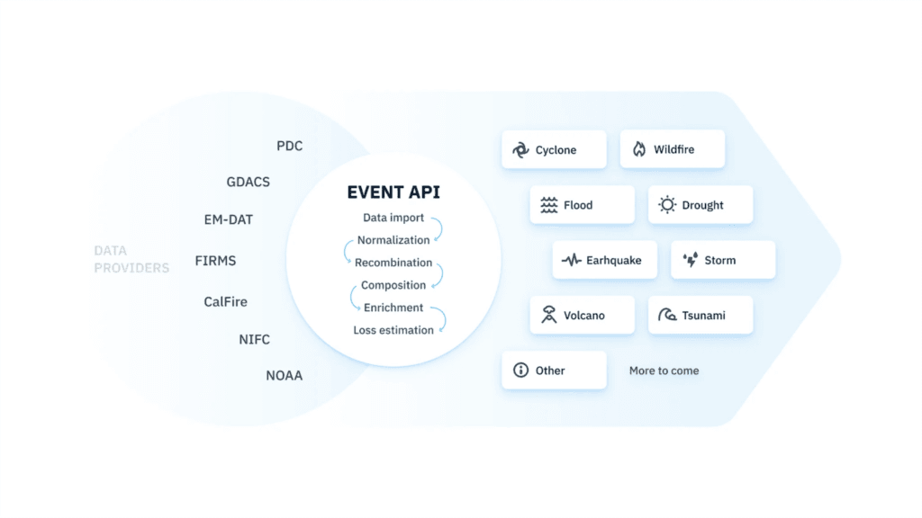


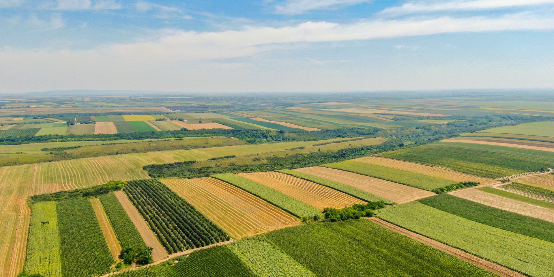


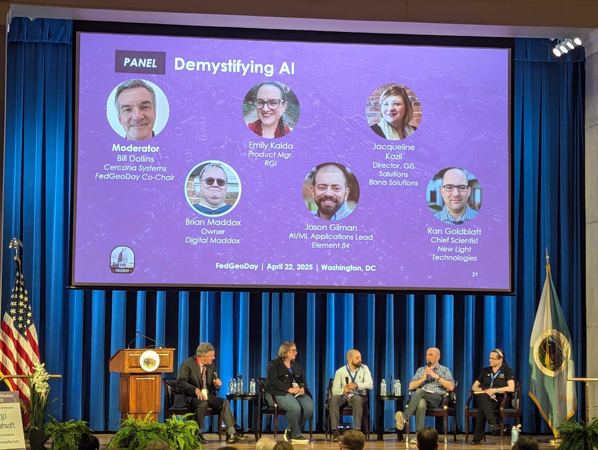
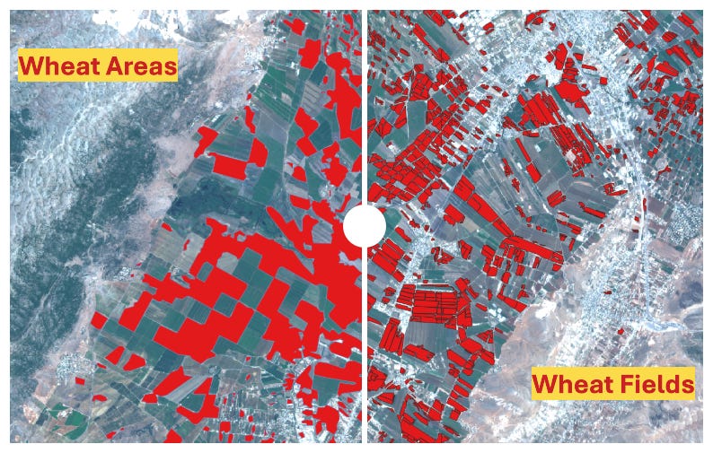


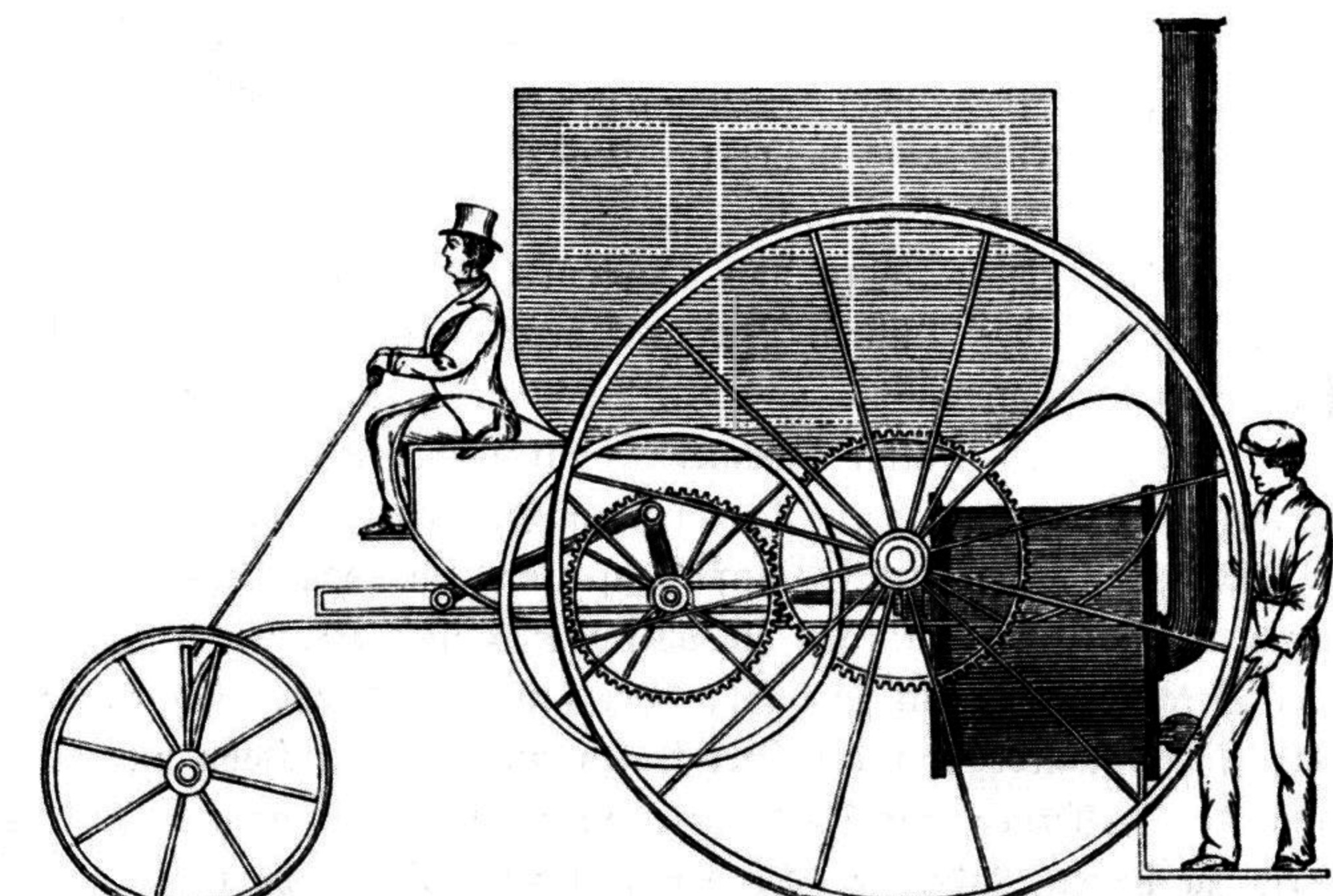

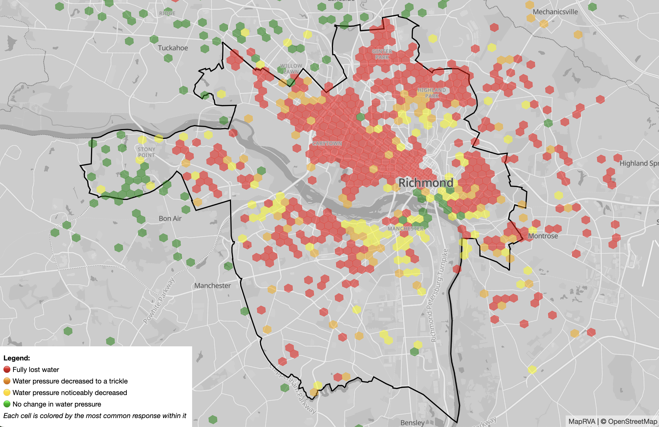
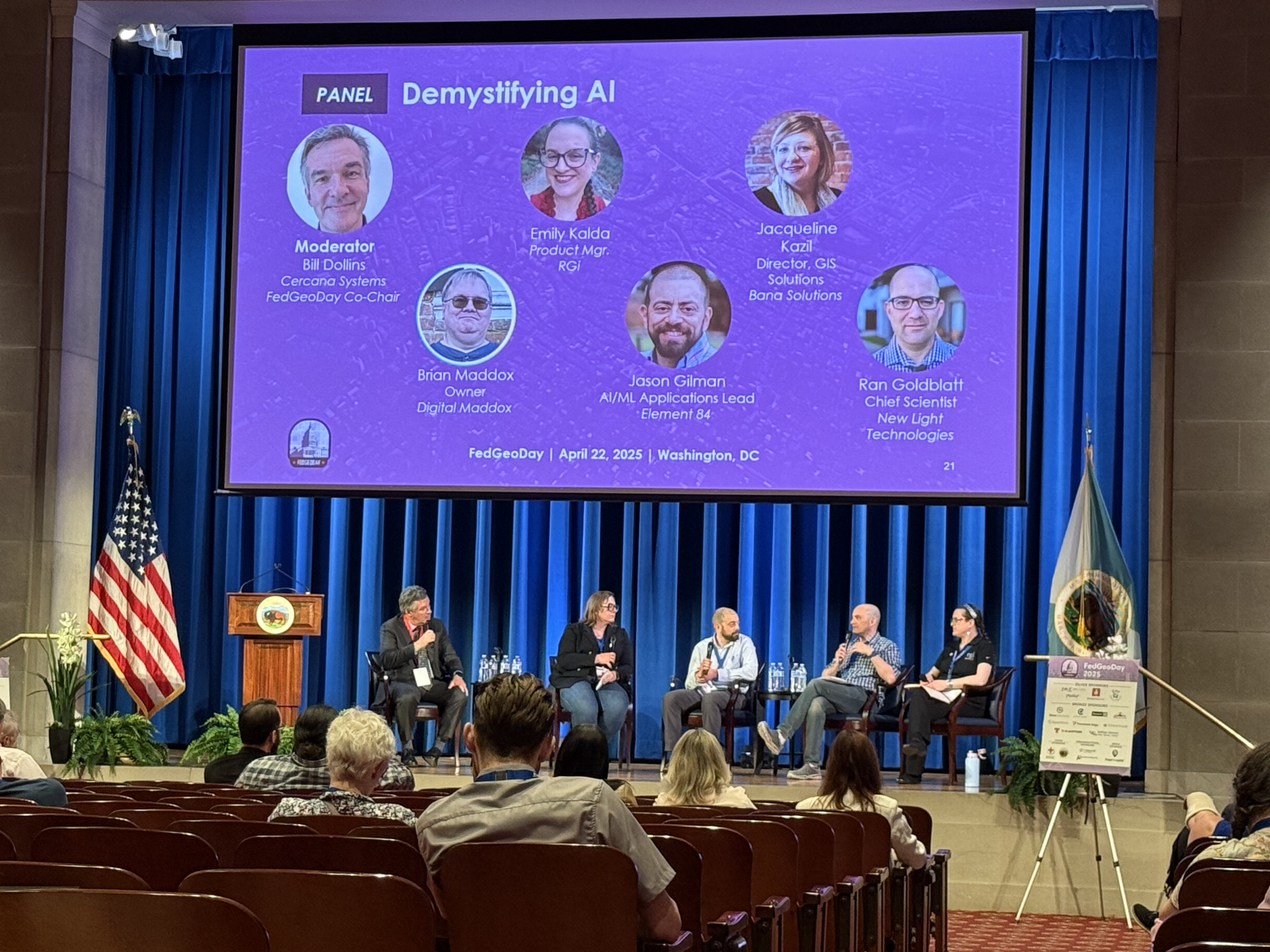


.jpg)


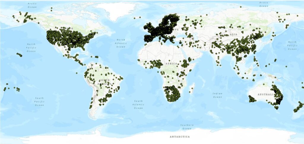


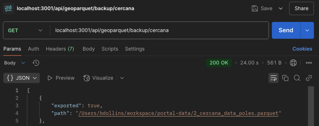

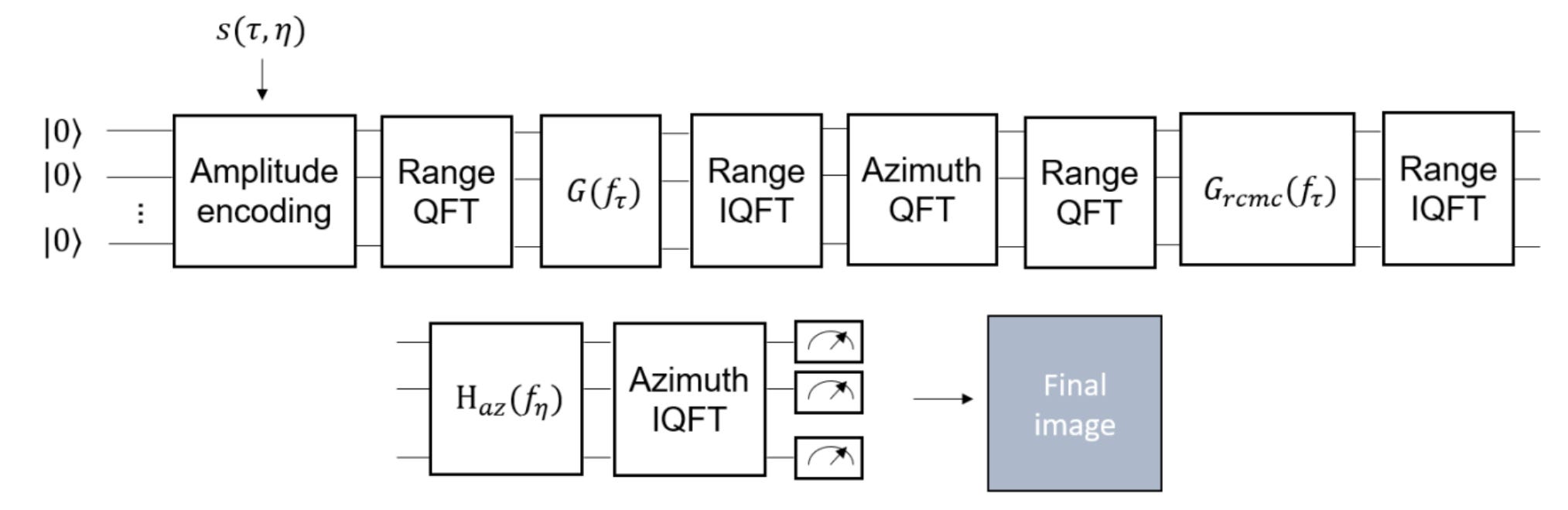


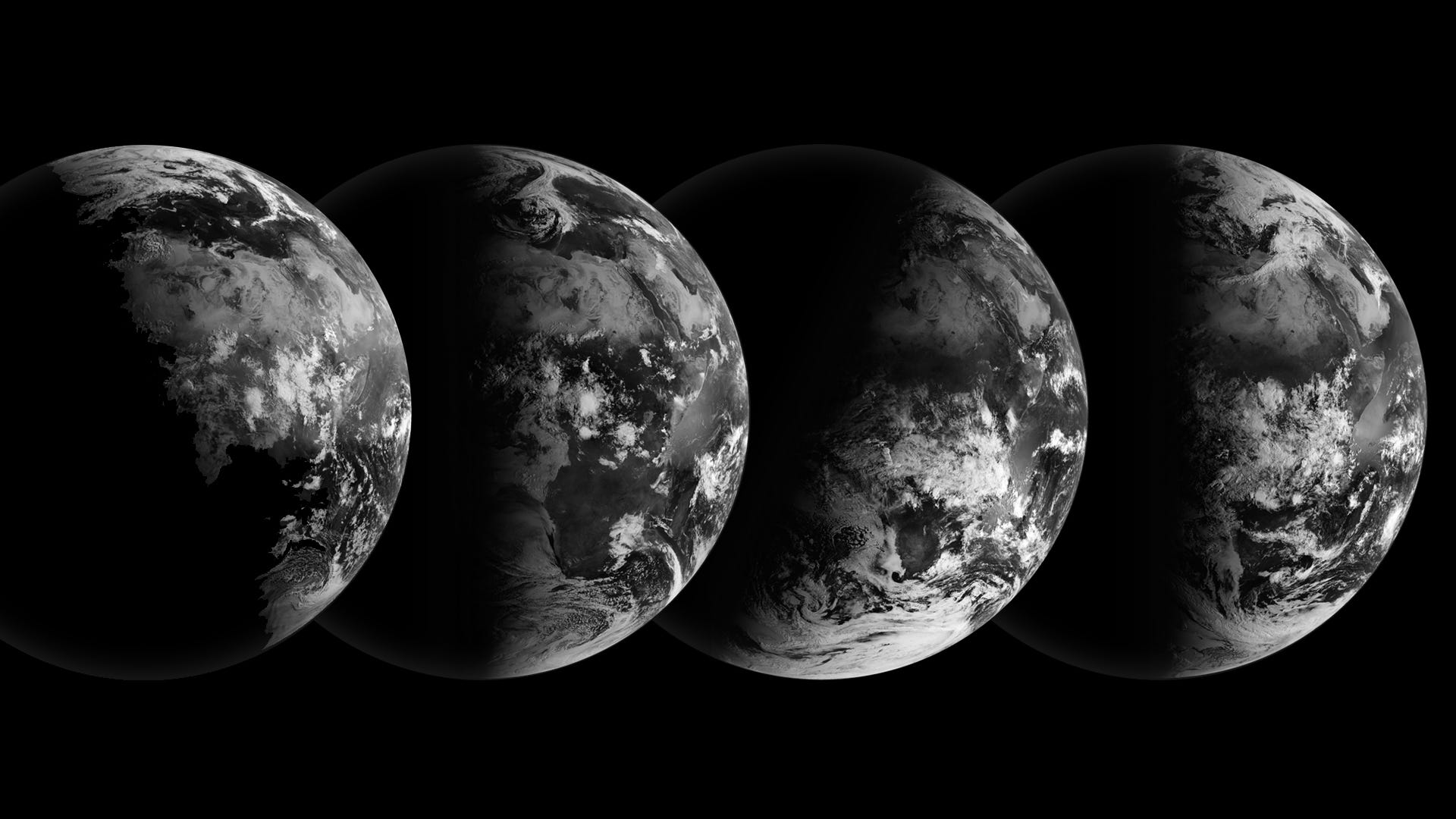
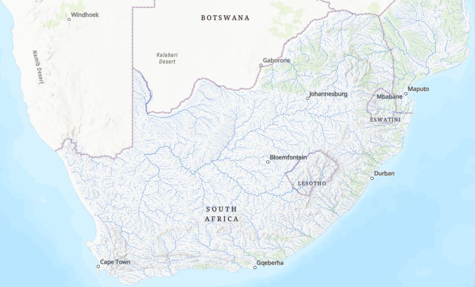
![Mergin Maps blog - [QGIS] Great Scott! Mergin Maps Plugin has a time machine](https://cdn.prod.website-files.com/64be358a4fb0e612b228bb9e/67daa339d7f7debfd82b7cf8_Image%207%20(1).png)